About numerics

This set requires numerical calculations. Write and submit your own codes in any language, e.g. Python scripts as .py text files or as PDF exported from Jupyter notebooks (not the notebooks themselves - the format is not readable in Quercus & we will not download and run your notebooks or codes!). Separate picture files are ok.

In a top comment section, sign your code, describe how you chose the value of timestep dt to assure an accurate solution. Put comments above all important lines of code, saying what they do & why. This way we I'll know it is your original code. If parts of the code are not yours, give credit to the author(s), cite the source; some points will be subtracted for that.

[15 p.] Problem 1. Precession in a funnel.

Two variables describing the particle are r(t) and φ(t). The first is the distance from the axis (not a 3-D distance from the bottom of the funnel). The third coordinate is then z = ξ r, where ξ = tan α, because the particle is always on the surface of the funnel.

Those of you who know Lagrangian mechanics from PHYB54, will be able to write the Lagrangian ℒ
[' and " are first and second derivatives over time and g = 9.81 m/s/s is the Earth's gravity constant]
ℒ (r,r',φ') = T - U = ½(1+ξ²) r'² + ½r²φ'² - g ξ r
and substituting it into Euler-Lagrange equations (click on the image, q := r or φ)

to derive the two equations of motion (derive them if you want, but that is not required & there will be no extra points for it):

φ' = L/r²
r" = a^-1 (L²/r³ - gξ)

Here, L = const. is the specific angular momentum [per unit mass of the moving test particle, r · velocity component perpendicular to (r,z) plane]. L = φ'r² is conserved because the funnel is axisymmetric. Consequently, there is no azimuthal force and no torque on the particle (Torque/mass = dL/dt = 0). Constant a = 1/cos²α = 1 + ξ² is a shorthand for the geometry of the funnel.

The dynamical system is conservative and frictionless. The motion starts at t=0 with sufficiently large φ' and L, but small (non-zero) r', so that the particle circulates inside the funnel, doing small up-and-down oscillation around a purely horizontal circulation. The system has a neutrally stable circular orbit (R,φ), R=const., for every r=R.

Your first task is to show analytically what φ'(0) is needed to yield a circular orbit for any starting value R = r(0), and what is the value of L(R) for the circular orbit. That φ' is the azimuthal angular frequency of the circular motion, as well as the average azimuthal speed of a nearly-circular motion: ω_φ = φ'. (There is also an associated period of azimuthal circulation 2π/ω_φ, but let's just calculate ω_φ.)

Next, sketch the acceleration r"(r) and the effective potential Φ(r) in which the autonomous r-motion with constant L takes place. The gradient -dΦ/dr is the r.h.s. of r-equation.

What is the frequency ω_r of small radial oscillations? Compute ω_r² either as -1 times the slope at which acceleration r"(r) crosses the r-axis or as the curvature of the potential (∂_r)²Φ.
[Think of a harmonic oscillator r" = -ω²r, and its quadratic potential Φ=½ω²r², where ω²≡ω_r² equals both the second derivative of Φ and the negative slope of r"(r) at the fixed point r*=0 - but the relation is general! Incidentally, small oscillations around equilibrium of any system governed by Newtonian dynamics are approximated very well by harmonic oscillator, because all minima of potential locally look like a parabola]

The difference Δω = ω_φ - ω_r of the radial and azimuthal frequencies is the angular speed of precession of the orbit. If non-zero, the orbit looks like an ellipse turning in space, or rosette, i.e. it self-intersects in (r,φ) plane. If Δω < 0 then the orbit gradually rotates in the direction opposite to the sense of orbital motion, otherwise in the same direction.
Find analytically the funnel angle α for which there is no precession. In such a funnel, test particle exerting small deviations from circular motion will repeatedly pass through the starting point and its orbit is closed and periodic.

SOLUTION

2. Frequency of small radial oscillations:
Φ = a^-1 [½L²/r² + ξg r]
has a minimum at r=R, force is zero (Φ'=0), and where the curvature is entirely due to the centrifugal barrier:
ω_r² = Φ"(R) = (3/a) L²/r⁴ = (3/a) φ'(R)² = (3/a) ω_φ².
3. Given that a = 1/cos²α = 1 + ξ², the radial to azimuthal frequency ratio is
ω_r/ω_φ = (3/a)^1/2 = [3/(1+ξ²)]^1/2 = 3^1/2 cos α.

4. The difference between the radial and azimuthal frequencies is the angular speed of precession of the orbit. There is no precession when ω_φ = ω_r, i.e. when cos α = 3^-1/2, or when α = arccos 3^-1/2 = 54.7356°.

Many commercially sold funnels have α = 60° and would produce ω_φ > ω_r, shorter azimuthal than radial period of motion, and thus precession with maximum distance points marching in the direction of motion (prograde precession). By experimentation, you can observe that this is also true of a rolling motion of a small ball inside such a funnel.

[15 p.] Problem 2. Numerical calculation of motion in a funnel

Compare that solution with the solution in case of either α = 60° or α = 45° (pick one value you like). Do you find agreement of the numerical precession speed with its analytical calculation in that case?

Write and submit your own code or Python script (see comments on numerics above). For clarity, show the trajectory seen from the top, i.e., the orbits should be shown in Cartesian (x,y) coordinates, not in polar coordinates, or as separate functions r(t) and φ(t).

[30 p.] Problem 3. Trajectory starting near L2 Lagrange point in Hill's equations

To remind you: negative x axis points to toward the star, and we study the planar motion of test particle in the Cartesian coordinates with rescaled length. Coordinates (x,y) are in units of Hill sphere radius (Roche lobe radius) $r_L= (\mu/3)^{1/3} a$, where $a$ is star-planet distance and $\mu =$ planet mass / (star+planet mass) $\ll 1$.
The beauty of Hill's equations is that they apply to any small planet, so the particular value of $\mu$ and $r_L$ is unimportant, and results in the same trajectory in rescaled coordinates. Here are the Hill's equations: $$ \ddot{x} = -3 \frac{x}{r^3} +3x + 2\dot{y} $$ $$ \ddot{y} = -3 \frac{y}{r^3} - 2\dot{x} $$ where $r^2=x^2+y^2$. Evidently, they are quite nonlinear because of $r^{-3}$.
Time drivatives are over a nondimensional time $t$ (unit of this time corresponds to time it takes the planet to turn 1 radian around the star). The meaning of the right-hand side terms has been described in the quasiblog. We already know that the positions of two fixed points are $(x^*,y^*) = (\mp 1,0)$. We call them Lagrange points L1 and L2. One being a mirror reflection of the other, they have the same stability properties, and the same eigenvalues $\lambda$ and eigenvector directions.

A [5p]. Prove the constancy of Jacobi energy:

$$E_J = \frac{1}{2}(\dot{x}^2 + \dot{y}^2) -\frac{3}{\sqrt{x^2+y^2}} -\frac{3}{2}x^2 $$ by explicitly evaluating the full time derivative $dE_J/dt$, and showing that it vanishes. Don't forget about the inner derivatives!

B [25p]. Numerical trajectory

Notice that we have four variables: $x,\dot{x},y,\dot{y}$. So we have a 4-D dynamical system. Program one of the many methods for solving the dynamical equations. Preferably use the leapfrog scheme (looks quite like Euler scheme when the starting velocity is zero). If you use someone else's software (commercial/internet) to integrate the equations, state that and 25% of points for this section will be subtracted.

At the beginnig, set the constant timestep to $\Delta t \sim 0.05$. As you integrate the system in time, print out from time to time (printing in every timestep creates too much output on the screen, but if you don't mind..) the value of Jacobi energy. Make sure the $E_J$ you start with does not differ from the final value by more than $10^{-4}$, otherwise consider the trajectory inaccurate and repeat the whole calculation with a smaller timestep. State the satisfactory value of timestep and the relative E_J error you have obtained (this could be in the comments section of your code).

Compute the departure from point (1,0) toward the planet, the center of attraction at (0,0). If you place a fixed point at rest, it won't start moving. Therefore, begin from (x,y) = (0.9999,0.00005), and $(\dot{x},\dot{y}) = (0,0)$.

Continue integration of Hills equations until such time that the orbit goes around the planet about 7 times. If you extend the time, trajectory overlaps so much that it is hard to follow its course.

Plot the trajectory and overplot positions of L2 and the planet, as well as marker points of a different color and size distinguishing them from the trajectory curve, every 0.1 time unit. Such visualization helps to see the speed in addition to direction of motion at every point of particle trajectory. Overplot the eigenvector direction (-1,0.5399) found analytically in Etudes, using a dotted line. Submit your well-commented program.

Suggestions on graphics:
Try to plot the trajectory with 1:1 aspect ratio if you can, that is with equally sized units on x and y axes. In Python, one can precede plotting with command such as
fig,ax = plt.subplots()
and then plot both the line of trajectory: plt.plot(trajx.trajy), and/or overlay individual points (x,y) points via: plt.plt([x,x],[y,y],marker="."), and then do ax.set(aspect=1). Planet's position can be plotted like this: plt.plot([0,0],[0,0],"ro").

SOLUTIONS

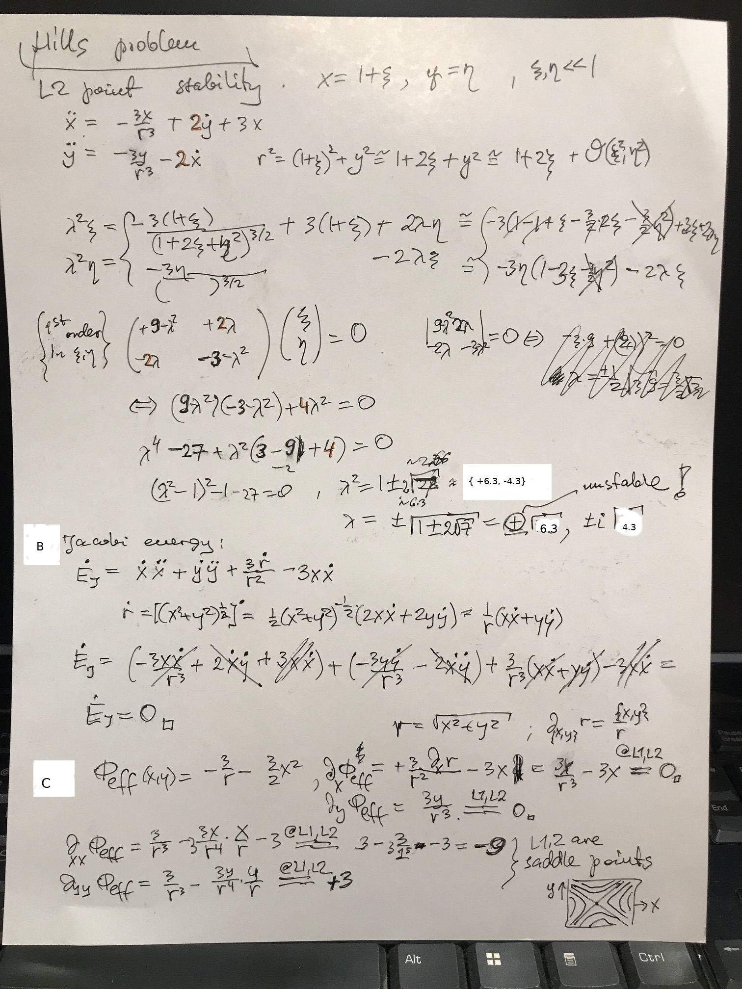
C. The effective potential is that part of the $E_J$ formula, which does not depend on velocity components (since that's kinetic energy part). $$\Phi_{eff} = -\frac{3}{r} -\frac{3}{2}x^2$$ At L-point, its first derivatives (forces or accelerations) vanish and the second derivatives (curvatures) along $x$ and $y$ axes have opposite signs. Curvature along x is negative (-9) and along y axis is positive (+3). See the calculation sheet above. That's a hallmark of a saddle point, and the equipotential lines would show this more clearly. Although equipotential lines of $\Phi_{eff}$ are not flow lines (along which $E_J = \Phi_{eff} + v^2/2$, not $\Phi_{eff}$ iteself, is constant), they do show boundaries of possible motion for a given value of the Jacobi constant. Equipotential lines are zero-velocity curves.

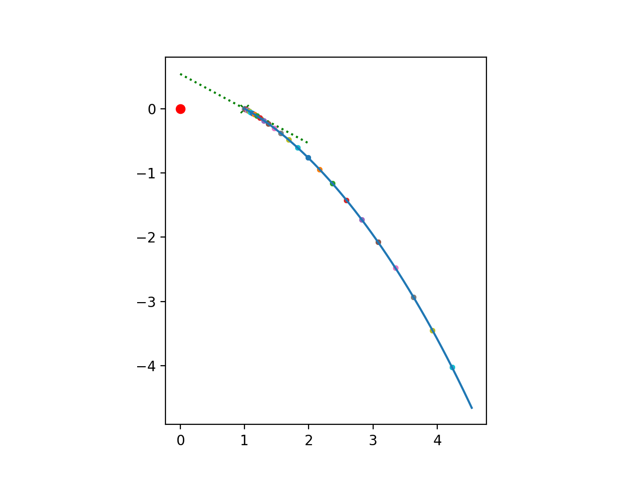
D. The trajectory plot shows the planet as a red dot, markers on trajectory are every Δt=0.1, i.e. every 1000 timesteps & eigendirection passing through L2 (dotted green line):

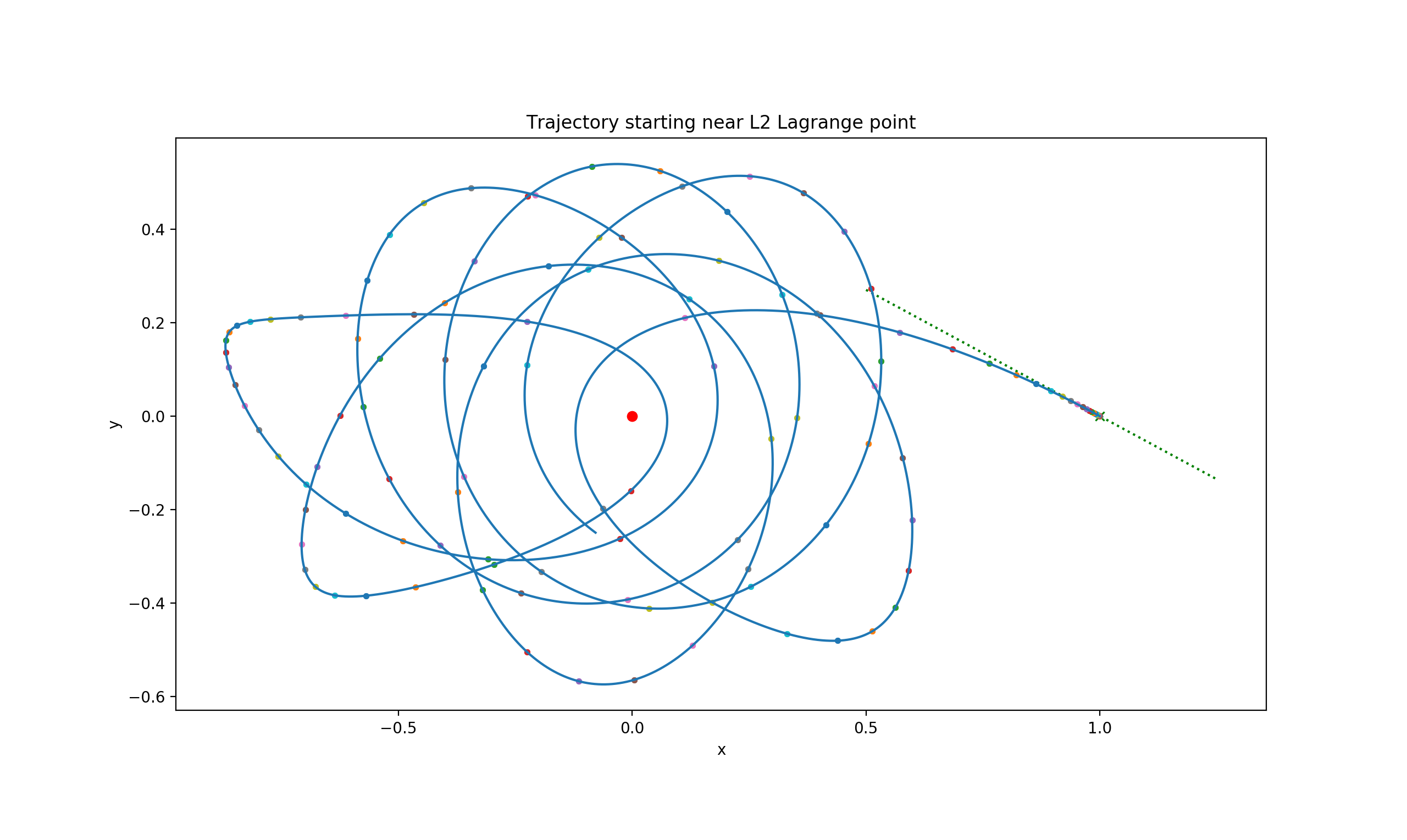
Notice that that a meaningful trajectory passing exactly through L2 could be constructed, but the time of passage would be infinite (critical slow-down at the unstable node).

[20 p.] Problem 4 - Rössler attractor

A. Is this system a chaotic attractor?

Starting from starting point $x=y=z=1$, numerically evolve the system for $a=0.3$, $b=0.2$ and $c =6$.
Use numerical integrator of your choice (write your own script or program and enclose it as a file, cf. remarks on numerics at the beginning of assignment). Recommended method is Euler method with short time step $\Delta t = 10^{-3}$. Continue up to time $T > 50$, large enough to clarify the bahavior and illustrate the chaotic or non-chaotic behaviour clearly.

Plot the trajectory in the projection on $(x,z)$ plane (i.e. ignore $y$ while plotting). Then ignore $z$ and produce another plot of $(x,y)$ projection.

B. Bifurcation.

Vary the parameter $c$ in the range $0 \lt c \lt 20$. Observe bifurcations (jumps in behaviour), describe your results and illustrate with just a few plots, included in solutions file or clearly described, if you submit separate figures.

C. Lyapunov exponent.

Adopt $a=0.2$, $b=0.2$ and $c =5.7$ and create a variant of your code to follow two different trajectories ($x_1,y_1,z_1$) and ($x_2,y_2,z_2$) at the same time. Start the 2nd trajectory with $x = y = 1$, and $z = 1- 10^{-6}$, and plot the 3-d distance between the trajectories as a function of time. Use log-linear scale, that is plot decimal logarithm of $D = ||(x_1,y_1,z_1)- (x_2,y_2,z_2)||$ vs. time. From the plot, estimate the Lyapunov exponent $\lambda$. Desregarding little wiggles, we expect $D(t) \sim \exp(\lambda t)$.