PHYD38. PROBLEMS #4 with partial solutions
[25 p.] Problem 4.1. Cubic maps, analytically
Consider the following cubic discrete map parametrized by c = const.
xn+1 = f(xn) = c xn - xn3
where x,c = real numbers.
Starting from x0, we are interested in asymptotic behavior of the
sequence of x's. (If you try it on a calculator, see if choosing a positive vs.
negative x0 value, and absolute value change the outcome
after some initial steps.)
A.
Find the fixed points of the map x*(c) depending on constant c.
For what values of c do they exist and what is their stability?
Sketch the bifurcation diagram x*(c) of period-1 fixed points.
B.
As it happens with many nonlinear maps, you will encounter a bifurcation.
You may suspect that bifurcations continue and lead to period doubling
at characteristic values of c.
Support this suspicion by writing f2(x) = f(f(x)) and formulating
equation for its fixed points. This will be a very high-order polynomial
equation, but after factoring out the common terms, you will be able to show
that the factored terms are the same low-order polynomials that you encountered
while hunting for period-1 fixed points. They multiply a polynomial of
still high (but lower) order, whose zeros are period-2 cycles.
Pieces pointing to period-1 orbits in the f2
polynomial are always present in f2(x), because period-1 fixed points
also satisfy the period-2 fixed point condition, though are not the most
interesting parts when you search for doubled periods.
This is because, if x=f(x), then x = f(f(f(...(x)))) = fn as well.
Identify the factor in the high-order polynomial f2(x)
that specifically gives period-2 cycles via equation f2(x) = x.
For that factor, show that at the point where period-1 orbits eventually lose
stability, at the critical value c = c2, the factor also assumes a
value satisfying condition of existence of period-2. How many period-2 fixed
points follow from the equation if c slightly exceeds c2?
SOLUTION TO A and B
Since, f(x) = x(c-x x), there are up to 3 real fixed points.
x* = f(x*) =>
x*=0 (for any c),
or
x* = ±(c-1)½ (for c ≥ 1 only; there are no fixed points
of this kind for c < -1).
Are these 3 fixed points stable or repelling? Derivative f'(x*) must be between
-1 and 1 for the fixed point to be stable. In other words, |f'(x*)| < 1.
pt.1: x*=0. f'(x*) = c-3x*2 = c, so for -1 < c < +1
this point is stable.
pts.2&3: f'(x*) = c-3x*2 = c-3(c-1) = 3-2c, therefore stability
is assured in the range: 1 < c < 2.
We see a supercritical (i.e. gradual) pitchfork bifurcation at c=1.
When c crosses value 1 left to right, the stability of the first point
is gently transferred from x*=0 to two symmetric branches of the pitchfork,
described by equations c-x*2=1, or x*=±(c-1)½ .
At c > 2, we have unstable (repelling) fixed points
located at on a line x*=±√(c-1). The same happens on the x*=0 line
for c < -1,
Local analysis of bifurcation leading to period-2.
Suppose its impossible to do the polynomial factoring presented below,
or it's too difficult for some reason.
Here is a simplified and less general analysis that you still can do.
We want to explore the period-2 solutions present just to the right of the
points c=2 and x*=±1. These positions are the last semi-stable
fixed points of period 1. After c > 2, stability of the two square-root
branches vanishes.
For a fixed c > 2, let us denote the two asymptotic, alternating, values
of x as x1 and x2 as we've done before:
x2 = f(x1) = x1 (c-x12)
x1 = f(x2) = x2 (c-x22)
We know that neither of the x's is zero. So when we multiply the two equations
side by side, we are allowed to cancel x1x2 on both
sides of equation. This gives a nice, exact, condition for period-2 oscillation:
(c - x12) (c - x22) = 1.
We expect the period doubling to occur at c=2, and
x*(c=2) = ±1, and we want to locally
establish the relationship between the small deviations from those values, on
the c>2 side of the bifurcation. Let us show that the branches begin
symmetrically below and above the x*=1 line.
We assume x1,2 = 1 ±λ, and for the variable c, we adopt
a small, positive, and nondimansional deviation ε, like so:
c = 2(1+ε). We assume λ,ε ≪ 1.
Substituting into the (..)(...)=1 equation above, and after multiplication of
the parentheses and dropping all quantities cubic and higher in small
deviations, we get:
λ = ±[2ε(1+ε)]½
This is the correct lowest-order approximation to the period-2 branches near
the c = 2 bifurcation point. The period=2 braches are parabolae put on a side.
Unfortunately, this poor-man's analysis does not provide much information on
the precise shape of the branches further out, or where their stability ends.
A simple script in a python-like language IDL confirms the branching at c =2 :
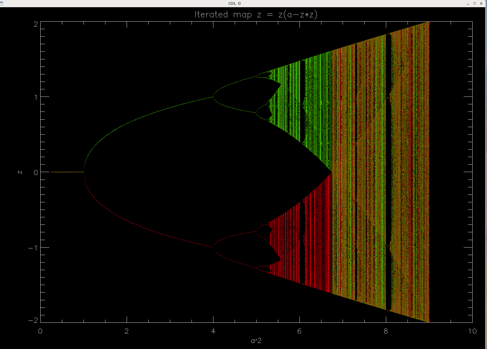
The x-axis is c2 (called a2), to show the large-c
region in more detail than low-c region. So the branching is at c2=1
and then 4. The next bifurcation seems to be at c2=5, but so far we
did not support that value (c = √5) with analytical calculaction.
Let's do that now.
Factorization: Advanced analytics.
Some of you provided a nice factorization of the rather cumbersome polynomial
equation that one gets when one explicitly searches for a fixed point of compund
f(f(.)) transformation. Factoring out things we know return the period-1
solutions for fixed pt., one gets factors that are returning the period-2 fixed
points:
[x2-(c+1)] [x4 - c x2 +1] = 0
The first term results in x* = ±(c+1)½ which is
an unstable branch, thus not seen in numerical orbit plots.
We can prove this by probing the derivative of f2(x) = f(f(x))
over x. Period-2 derivative equals f2'(x) =
f'(x1) f'(x2) [see Strogatz texbook or perform
the derivative].
Here, f'(x) = c-3x*2, therefore f2'(x1,2) =
= c-3(c+1) = -3-2c (same value for both fixed points in the form
x* = ±(c+1)½). We see that the derivative is less than -1
for all c > -1 that we are interested in □.
The polynomial in the second square bracket is the one that yields the stable
period-2 fixed point branches, oscillating forever between two fixed values:
x1,22 = c/2 ± [(c/2)2-1]½.
Notice that there are two root for squares of fixed points, so there
are a total of 2 pairs of 2 associated roots that oscillate between themselves:
numerics will show that the cubic mapping produces at c>2 the jumps between
the roots of different absolute value, but the same positive or negative sign.
Let's check the theoretical stability. This will allow us to find the
exact bifurcation point into period-4 branches. If we
denote R = [c2/4 - 1]½, then
f2'(x1,2) = (c-3x12)
(c-3x22) =
(-c/2 -3R)(-c/2 +3R) = c2/4 - 9R2 = 9 - 2c2.
Stability (incl. marginal stability)
is equivalent to |f2'(x1,2) | ≤ 1, or
4 ≤ c2 ≤ 5
or for positive c that we care about, c in the range from 2 to √5
inclusive. The corrresponding values of x* are square roots (with ± signs)
of the golden ratio (x1), and golden ratio minus one
(x2). Golden ratio is (√5 + 1)/2, check internet for
why it's an intersting number.
Here are the numerical results obtained with this
IDL script:
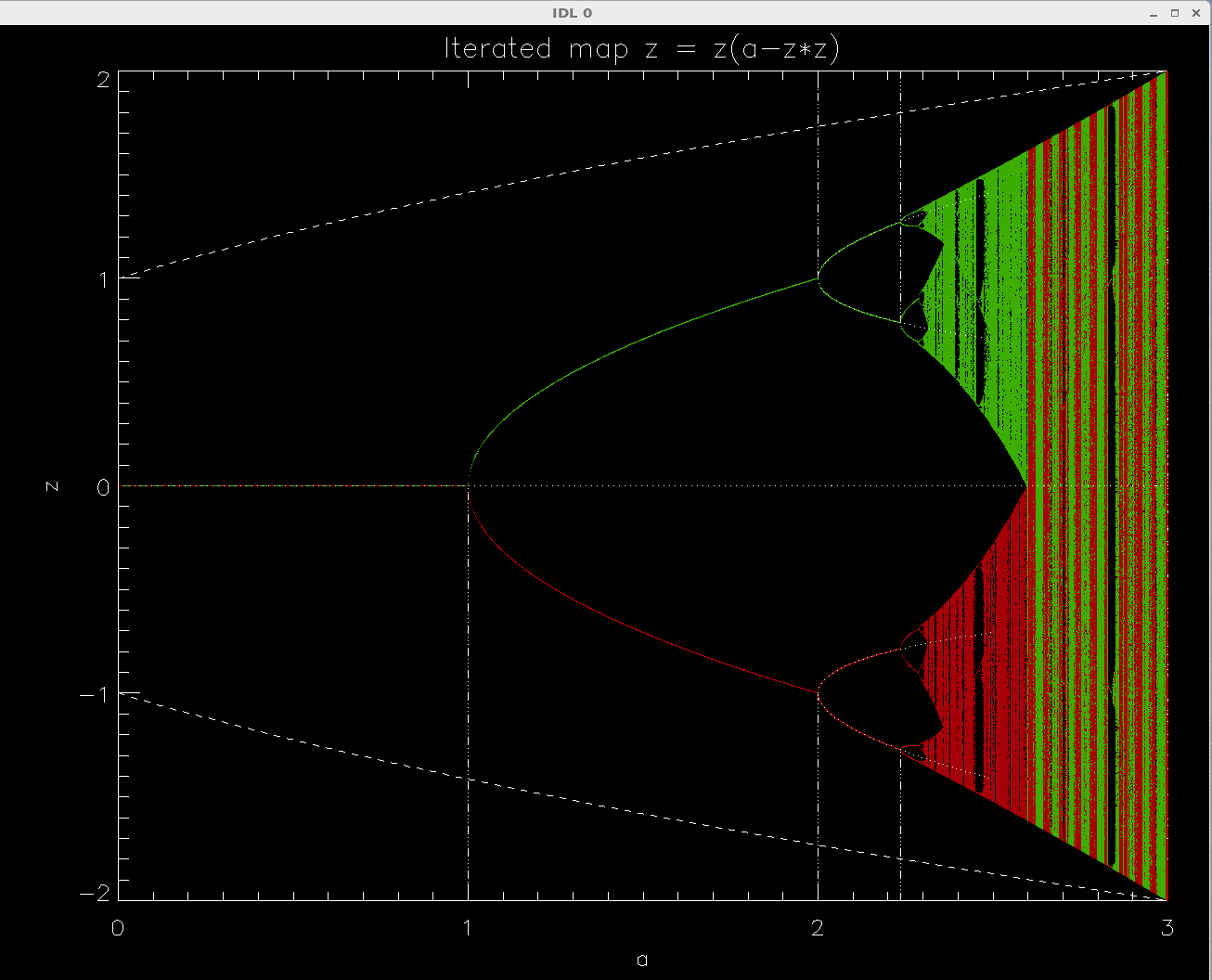
This is a plot of the numerical orbit diagram of iteration
xn+1 = xn(a - xn2).
Lower axis gives the values of parameter a, the same as c; vertical axis for
some obscure reason is called z instead x. Sorry.
Red and green points are obtained by starting the iteration from
x0= ∓0.2.
The theoretical curves are superimposed: the horizontal dotted line is the
unstable branch x* = 0, the dashed lines are unstable period-2 solutions
jumping between x* = ±(c+1)½ (notice how they eventually
collide with the chaotic but bound oscillations), and after the second
period doubling we see four fixed points in two pairs (red and green).
Results clearly show that the stability of the x*=0 branch ends at c=1, where
we get bifurcation into two branches of period-1 fixed points, both branches
being stable till c=2. This confirms our analytical work presented above.
C.
Consider a closely related, negative cubic map
xn+1 = f(xn) = -c xn +
xn3
where x,c = real numbers.
Find the map's fixed points x*(c), depending on constant c. For what values
of c do they exist and what is their stability?
Sketch the bifurcation diagram, speculatively also the period-2 orbits.
SOLUTION
In this case, fixed points are: x* = 0 (for every c), and x* =
±(c+1)½ (for c > -1).
f'(0) = -c + 3x*2 = -c, so the stability condition is the same as
for cubic map (c between -1 and +1 produces stable x*=0).
f'(±(c+1)½) = -c +3(c+1) =
3+2c, and stability criterion reads
-1 < 3+2c < +1 <=> -2 < c < -1.
Consequently, for c yielding a real nonzero x*, i.e. for c > -1,
there is no stability. All non-trivial period-1 branches are unstable.
The shape of bifurcation diagram is the same as in the cubic map, but
beyond the bifurcation point c=1 we already switch to the first period-2
oscillation.
Period-2 analysis shows close similarity with the analysis of cubic map
(sign of f reversed from the present). We can thus expect the
2x(period-2) solutions starting at c=1 and ending at c=2.
In contrast, the x = +x(c-x2) iteration has separate period-1
branches between c=1 and c=2, and no period-2 solutions there.
[25 p.] Problem 4.2. Cubic maps, numerical orbit diagrams
Use a software such as Python that allows plotting of separate colored points
in a graph. Write scripts to iterate the cubic and negative cubic maps
arising in the previous problem:
xn+1 = ± (c xn - xn3)
Either write two almost identical scripts for two equations, or have a
way to toggle the sign of r.h.s., in separate executions.
In each case, do the iterations for 2000 values of c spread uniformly in
interval c ∊ [0.5,3.5]. For consecutive c's, alternate the staring
points between x0 = -0.1 and +0.1, in order not to miss any
solution branches. Iterate 5000 times, but plot in the (c,x) plane points
showing only the second half of the sequence, to allow it to settle in
the final cycle(s) before plotting.
Whenever |xn| > 100, break the iteration.
Only plot x values in the range x ∊ [-2,2].
Plot the sequences starting with different x0 using two distinct
colors. With the help of your results of analytical study in 4.1, interpret
colors you see in different parts of the orbit diagram. Why are the two
equations showing similar features but different color patterns? Why does
neither plot continue past c=3; what happens if c>3 or c<-1?
Advice about plotting:
If you see that the points saturate the picture, i.e. are
overlapping, switch the symbols to smaller ones, even single pixels if necessary.
The horizontal axis of the orbit diagram is usually a linearly scaled parameter
a. But since most interesting small-scale features may be hidden in the
right-hand side of the diagram, to see them more clearly you may experiment
with showing c2 instead of c, on the horizontal axis (and label it
accordingly).
If you do that, interval 0 to 1 will take about the same amount of horizontal
space in the plot as the interval 2.8 to 3, that is you will effectively zoom in
on the r.h.s. of the picture. [In other applications, if you wish to expand the
view of the left-hand part of the horizontal axis,
you may wish to plot log(x) instead of x.]
BTW, nothing is more maddening than trying to understand figures with unlabelled
or unmarked axes, or undecipherably small axis labels, so always make sure there
is no doubt what you have plotted versus what, and in what range. Font size
in axis labels must be easily readable.
NUMERICAL SOLUTION of negative cubic map
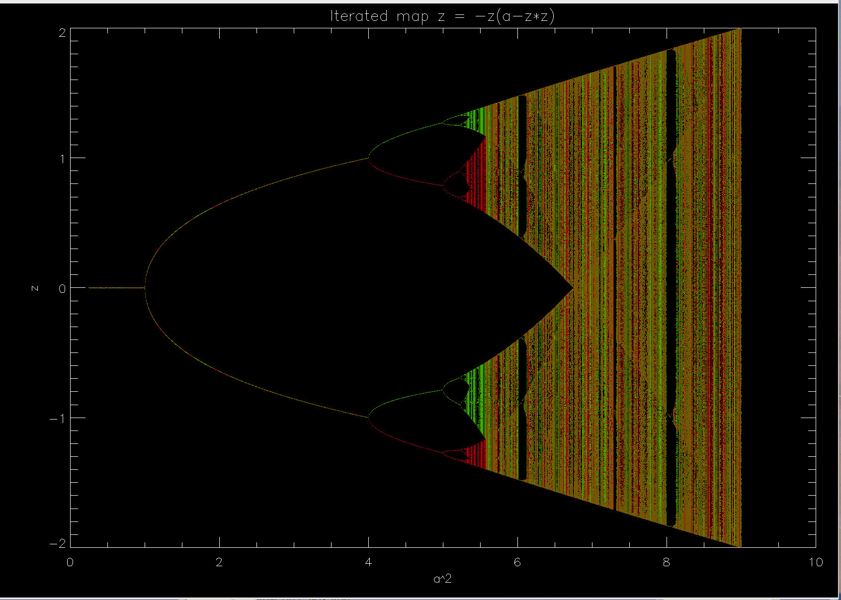
In this plot, horizontal axis is devoted to parameter a (but that's a wrong name,
it should be caled c). Iterated values
have been plotted against the square of the parameter, a2
= c2. This was done to effectively expand the more interesting
right-hand region of the plot, and compress the left-hand side.
The analysis goes along the same track as in the positive r.h.s. sign,
and incidentally many equations do not change ar all.
Fro any given c, similar points are visited but their stability may
be different. So what's different? Mostly that the
Why is there an abrupt end to all orbits at c=3?
For c>3 or for c<-1, the program does not generate anything interesting
(orbit diagram ends there). The explanation is that, just like in the normal
cubic mapping, there is an implied dashed line of repelling fixed points
x* = ±(c+1)½, running through the figure without
interaction with the cyclic or chaotic, but always limited-amplitude
oscillations.
But at c=-1 and c=3 the orbit diagram is colliding with the unstable &
repelling fixed points of cubic or negative cubic mapping, acquiring
their bad habit of repelling values to infinity. That's why we don't have
any |x*| > 2, such values would lie above the dashed line.
In fact, the fixed points do not vanish; they move off the real x-axis and
become complex numbers. We do not consider complex-valued iterations here, so
for us the orbit diagram has to end abruptly.
[25 p.] Problem 4.3. Fat and not so fat fractals.
In the lecture we discussed Cantor set (very "thin" fractal, a.k.a. Cantor's
dust). Then we saw Koch's snowflake built on the basis of an initial
equilateral triangle, which has a fractal boundary with infinite length,
but encloses respectable, finite volume, which one can compute by identifying
a geometrical progression in the sum of the
areas added in each iteration of the construction algorithm.
A. If the area of the starting triangle is equal 1, compute the area of Koch's
flake. To do this, write the formulae for: (i)
number Nn of sides after step n=1,2,3,... of the procedure,
(ii) length of each side after step n, (iii) area of each constructed (added)
little piece, (iv) total area added in step n, (v) total area added.
Notice: do not use trigonometry or formula for the area of the equilateral
triangle with known side. Proofs of this kind are readily found on internet
but any mention of factor ½√3 used in them will nullify the credit
for problem 4.3. Rely instead on the scaling properties: e.g., if a regular
solid object is scaled to 1/b its linear size, its area decreases by a factor
1/b2.
B. Similarly, compute the area of an inverted snow flake, object whose boundary
is constructed the same way as the Koch snowflake. While the snowflake grows
inside out, inverted snowflake grows outside in, as if ice was deposited on
an initially straight, smooth, wall of a triangular container. What percentage
of initial unit area is eventually found between the outside wall and the
fractal boundary?
C. Consider an even fatter object: a surface of square flake. It starts as a
square of unit area, and gradually grows on each side, in the outward
direction, an equilateral extension. Each boundary piece has its middle
1/3 taken out and replaced with 3 new pieces of 1/3 length, put at right
angles to neighbors.
Using procedure outlined above, find the length of the corrugated perimeter,
and the area of the square flake. What is the shape of the boundary? That is,
what shape is the box into which we can efficiently fit the square flake,
and what is its size?
D. What is the similarity and box dimension of the boundary of the 3
objects described in points A-C? And what dimension d has the body of yet
another object, which is constructed just like in section C, but in each
step also has the middle 1/9th of each full square removed?
SOLUTIONS to 4.3
A. Let's call the building of initial triangle (area=1) step n=0.
Number of sides Nn = 3 4n; Ln =
3-n; area of one little triangle added in step n is
an = Ln2. This is a somwhat strange
set of area and length units, since the n=0 step has length
AND area equal 1, but it's very useful here.
Therefore, the total length is
L = lim(n→∞) NnLn = ∞
Total area added in step n to Nn-1 sides is
dAn = Nn-1 an = 4n-1
31-2n. The total area added equals
sum of dAn from n=1 to ∞, or
Σ{n=1...∞}
4n-1 3-1-2(n-1) = 3-1
(1+4/9+(4/9)2+...) = (1/3)/(1-4/9) = 3/5.
Thus the Koch triangle has a total area equal 1 + 3/5 = 8/5 = 1.60
B. Inverted snow flake has number of sides
Nn = 3 4n, Ln = 3-n, and the
area of one little triangle added in step n is an =
Ln2,
therefore the total length L = lim NnLn = ∞,
just like Koch's triangle.
Area added in step n = dAn = Nn-1 an
as before, so the total area of ice (or icicle) grown inside the container in
all the steps will be the same 3/5 as in Koch's flake.
The only difference is that this is the whole area of the object, 3/5.
C. Square flake has Nn = 4 5n,
Ln = 3-n,
and the area of one little square added in step n =
an = Ln2.
Therefore the total length L = lim NnLn = ∞.
In step n, the added area is
dAn = Nn-1 an = 4 5n-1
3-2n = 4 5n-1 3-2-2(n-1) = (4/5)
(5/9)n.
Therefore, the total added area is
ΔA = (4/5) Σ{n=1...∞} (5/9)n = 1.
Total area of square snowflake is thus A = 1 + 1 = 2.
The bounding shape within which the flake is growing is a bigger
square turned by 45 degrees. Its side is √2 and area equals 2. This
can be seen from a good drawing of he first few steps of procedure.
A good drawing has many little squares touching each other.
We see that the area of the bounding shape is exactly the same as
the total area of the square flake: there is no empty space (area) left
within the object. But the object cannot be considered simply a bigger
square, since it has a complicated boundary of infinite length.
We call it a fat fractal.
D.
Let's start from the square snowflake (area).
Similarity dimension is poorly defined, since increasing size of the flake
by a factor of 2 does not give us M copies of the smaller flake. Because
of the solidly covered inner part, the object is not strictly self-similar,
only its boundary area looks self-similar (to which I'll return).
What about the box dimension? It is well defined.
At n≫1 the area of the object becomes really close to 2 units,
while the covering objects are squares with side
ε = (1/3)n, and area ε2 each.
We need almost 2/ε2 of them to cover the n-th stage
of the construction of the square flake.
The needed number is Mn = 32n.
By definition, box dimension equals
d = lim{n→∞} ln Mn/ ln[1/ε] =
lim{n→∞} ln 32n/ ln(3n) = 2.
So judged by the box (covering) dimension, the object is not a fractal at all!
But didn't we say that it is surely a fractal, since it has an infinite border
length? So what's going on?
The solution to this paradox is that there are two very
different things: the fractal which is made of linear segments and the
interior of it, which has a nonzero area.
The first is self-similar on different scales, and has fractional similarity
and box dimensions, ln(4)/ln(3)=1.2618..
in case of the Koch triangle and inverted Koch triangle, and ln(5)/ln(3)=1.4649..
in case of the square snowflake,
because using 3x shorter pieces as measuring sticks or boxes or spheres
(linearly smaller boxes), we need to use 4 or 5 of them, on the same part of
the object. The second type of object, the inside area, does not necessarily
need to be a fractal, is not strictly self-similar, and technically it isn't a
fractal because the covering (box) dimension is 2.
[25 p.] Problem 4.4. Which sequences?
Which sequences $z_n$ ($n>0$), all convergent to a constant $z_*$, does
the Aitken process accelerate correctly? Consider these (idealized!) types of
convergence, with $z_*,a,b$ being complex constants:
1. $z_{n} = z_* + a\, e^{-b n}$ (exponential)
2. $z_{n} = z_* + a\, n^{-b}$ (power law)
3. $z_{n} = z_* + (a/n)\,\sin(b \,n) $ (neither/combined)
Look at the last two
Etudes , use two methods, one treating $n$ as integer variable, the
other as a continuous variable (like $x$). Perform analytical and/or numerical
investigation (analytical is more impressive when it gives simple results,
but numerical is more widely applicable and informative, in the end :-)
If you get stuck with difficult analytics, employ numerics.
Solutions 4.4
1. Exponential case
This is a very often found type of approach to a fixed point, for instance
in a continuous $\dot{x} = f(x)$ dynamical system, when $f(x_*)=0$ and
$f'(x_*) \lt 0$.
Treating $n$ as continuous variable, it is easy to show by direct substitution
that $A(n) = z(n) - z'(n)/z^{''}(n) = z_*$ (perfect acceleration):
$$ z(x) = z_* +a\, e^{-b n} $$
$$ z'(x) = (-b)\, a\, e^{-b n} $$
$$ z''(x) = b^2 \,a\, e^{-b n} $$
$$ A(x) = z - (z')^2/z'' = z_*.$$
Discrete case works likewise. Immediately, we get $z_*$ from the first triplet
of consecutive terms we encounter in an idealized exponential series (any
triplet, in fact):
$$ z_n = z_* + a\, e^{-b\,n}$$
$$A_n = z_{n} - \frac{(z_n - z_{n-1})^2}{z_n -2 z_{n-1} +z_{n-2}} =
\frac{z_{n}\,z_{n-2}-z_{n-1}^2}{z_n -2 z_{n-1} +z_{n-2}}.$$
We will use the first equality.
$$A_n = z_* + a\, e^{-b\,n} - \frac{(1- e^b)^2}{1 -2 e^b + e^{2b}}\,a\,
e^{-b\,n} = z_* + a\, e^{-b\,n} - \frac{(1- e^b)^2}{(1 -e^b)^2}\,a\,
e^{-b\,n} = z_*.$$
Very nice. No need and no way to improve on that result (neither Aitken nor
further Shanks transforms work, if the sequence has a linear plot of the values,
for instance if it is constant, then the denominator is zero).
Comment: Recall the complex self-exponentiation series for $..i^{i^{i^i}}$.
We did get a good acceleration of convergence. That exponentiation process
works less efficient than in purely exponential convergence, but better
than in a power-law case.
2. Power law case
It's not as great as acceleration of exponential convergence.
You appreciate that fact especially if you start with the discrete case
of Aitken process:
$$ A_{n} = z_{n} - \frac{(z_n - z_{n-1})^2}{z_n -2 z_{n-1} +z_{n-2}}$$
where
$ z_{n} = z_* + a\, n^{-b}, $ $ z_{n-1} = z_* +a\, (n-1)^{-b}, $
$z_{n-2} = z_* + a\, (n-2)^{-b}$
$$ A_{n} = z_*+a\,n^{-b} -\frac{[1 -(n-1)^{-b} n^b]^2}{1 -2(n-1)^{-b}n^b
+(n-2)^{-b}n^b } \,a\, n^{-b}$$
$$ A_{n} = z_* -\frac{ \left( \frac{n}{n-2}\right)^b
-\left(\frac{n}{n-1}\right)^{2b}} {1 -2\left(\frac{n}{n-1}\right)^b
+\left(\frac{n}{n-2}\right)^b } a\, n^{-b}$$
We can study the behavior for $n\gg 1$ by expansion $\frac{1}{1+\epsilon} =
1-\epsilon +\epsilon^2-\epsilon^3 +...$
For instance, with error of order $O(n^{-4})$,
$$\left(\frac{1}{1-2/n}\right)^b = [1+2/n +4/n^2+8/n^3 +...]^b =
1+2b/n +2b(1+b)/n^2+
...$$
$$\left(\frac{1}{1-1/n}\right)^b = [1+1/n +1/n^2+1/n^3 +...]^b =
1+b/n +b(b+1)/(2n^2)+... $$
$$\left(\frac{1}{1-1/n}\right)^{2b} = 1+2b/n +b(1+2b)/n^2+...$$
Therefore
$$ A_{n} = z_* + a\, n^{-b} \frac{1}{1+b} [1+O(1/n)]. $$
We see that the convergence is improved a bit over the original $z_* +an^{-b}$,
the deviation from the fixed point decreased to $1/(1+b)$ of the previous one,
which is never a very substantial factor.
Consider now the analytics in the continuum case. The math gets much easier.
We change power $-b$ to $-p$, because, perhaps, we will get other formulae,
not to be confused with what's above.
$$ z(x) = z_* +a\, n^{-p} $$
$$ z'(x) = -p\, a\, n^{-p-1} $$
$$ z''(x) =(p)(p+1) \,a\, e^{-p-2} $$
$$ A(x) = z - (z')^2/z'' = z_* + a\, n^{-p}\,\frac{1}{1+p}.$$
That's it, we got the same factor with less effort.
So the Aitken sequence of power-law type approach to the fixed point, at every
$n$, simply slashes the distance from it by a factor $1/(1+p)$. Example.
Suppose we have a sequence of leapfrog calculations of some given length of
trajectory of a dynamical system, with $n$ denoting the numer of subintervals
(time steps in the integration of the ODEs). Leafrog is a second-order
integrator, so $p=2$. The gain is a factor 3 (3 times smaller error for every
$n$, not 3 times fewer steps for a given accuracy).
The convergence of power-law series is aways moderately slow. We'll need a
factor of $\sqrt{3}$ fewer steps to reach the same accuracy. Considering that
computational effort (number of operations) needed to achieve $n$ steps
grows proportionally to $n$, and may be considerable, the total amount of work
is much lower if we only have to do only $1/\sqrt{3}$ of the work.
Shanks transform, on the other hand, can extend this gain by repeatedly cutting
down the error.
Click on this figure, presenting the discrete case, power-law series and its
acceleration :
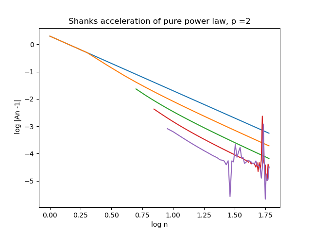 Aitken series of the original blue series is shown in orange. Further Shanks
transforms (iterations of Aitken) are shown in green, red, and purple. Iteration
runs to $n=60$. It makes little sense to continue Shank's transforms, because
the recursive differentiation is always bound to amplify any noise
(e.g. due to arithmetic inacuracy of the last digits, especially in denominator,
where we subtract very similar quantities from one from another). But we got a
nice result despite the same power law $p$ in all curves, the same
slopes. Original series, after 60 steps, gets us merely 3 accurate digits of
$z_*$ (deviation is $10^{-3}$). Power laws converse slowly. But if we do only
1/6th of the work and stop at $n=10$ (log $n$ = 1.00 in the figure), from
Shanks's process we correctly infer the same number of 3 accurate digits, and
with 1/3rd of the original work ($n=20$) we can achieve 4 accurate digits.
Aitken series of the original blue series is shown in orange. Further Shanks
transforms (iterations of Aitken) are shown in green, red, and purple. Iteration
runs to $n=60$. It makes little sense to continue Shank's transforms, because
the recursive differentiation is always bound to amplify any noise
(e.g. due to arithmetic inacuracy of the last digits, especially in denominator,
where we subtract very similar quantities from one from another). But we got a
nice result despite the same power law $p$ in all curves, the same
slopes. Original series, after 60 steps, gets us merely 3 accurate digits of
$z_*$ (deviation is $10^{-3}$). Power laws converse slowly. But if we do only
1/6th of the work and stop at $n=10$ (log $n$ = 1.00 in the figure), from
Shanks's process we correctly infer the same number of 3 accurate digits, and
with 1/3rd of the original work ($n=20$) we can achieve 4 accurate digits.
There are very good symplectic integrators of 4th order (not RK4, it is not
symplectic). They have $p=4$ and with the cleverness of nonlinear transforms,
we can do just 10 or 12 integrations with different number of steps (equally
spaced), and derive from the Shanks process a much much more accurate result
than if we spent the same computational resources than without it. Click on
this figure, presenting the discrete case, $p=4$ series and its acceleration:
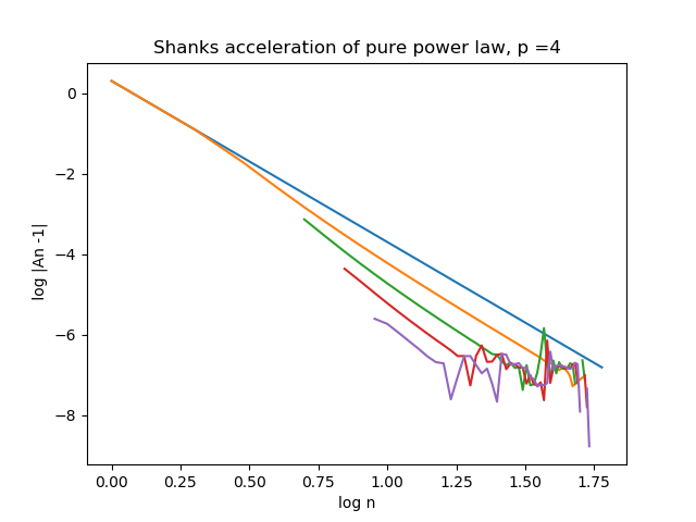 It looks like we can spend 5 times less computing power to find 6 accurate
digits, by iterating Aitken transformation.
It looks like we can spend 5 times less computing power to find 6 accurate
digits, by iterating Aitken transformation.
3. Mixed or combined case of exponential and power law-type approach to
fixed point
$$ z(x) = z_* +\frac{a}{n} \sin b\,n\,,$$
$ z'(x), z''(x)$ are both a jumble of terms, but we can still get the $A_n$
and it doesn't look encouraging:
$$A(x) = z_* + \frac{a}{n\,\sin b n},$$
a function with singularities, which does not, strictly speaking, converge.
This is confirmed by numerics.
Click on this figure, presenting the discrete case, power-law series and its
acceleration :
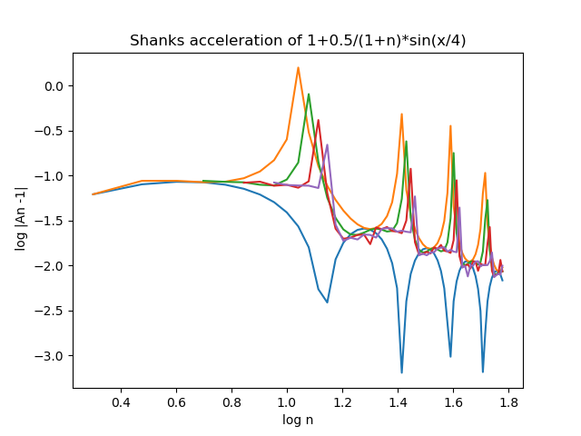 Yep, it's a disaster. Aitken's transform is less accurate a predictor
of $z_*$ than the original $z_n$ series. (Did you know "disaster" in medieval
Latin of astrologers meant 'wrong stars', i.e. wrong alignment of stars, in our
case the asterisk in $z_*$).
Yep, it's a disaster. Aitken's transform is less accurate a predictor
of $z_*$ than the original $z_n$ series. (Did you know "disaster" in medieval
Latin of astrologers meant 'wrong stars', i.e. wrong alignment of stars, in our
case the asterisk in $z_*$).