Assignment 1, PHYD57

Due date: 22 Sep (Sun) at 11:59 pm

Problem 1.1 [30 pts] Ballistic motion in air

Write a procedure that takes $\alpha$ as input, and returns:
(i) maximum height $h$ in meters,
(ii) the range $R$ in meters [the ball touches down at point $(R,0)$] and
(iii) the ratio of $x_h/R$ (to judge the asymmetry of trajectory's shape). Here, $x_h$ is the $x$ value at which the height is maximum.

If the motion takes place in vacuum, the problem has a simple analytical solution for (i)-(iii). Please derive it. Show that, in vacuum, maximum range $R$ is obtained with $\alpha_m = 45^\circ$ (evaluate $R$ and $h$ in vacuum), and the trajectory is a symmetric, inverted parabola ($x_h/R = 1/2$).

Numerical calculation is necessary when the tennis ball moves in air of standard atmospheric density $\rho = 1.225$ kg/m$^3$. Do not try to find analytical solution, since it is not known, except for very special $\alpha$, like 0 or 90$^\circ$. Please integrate the equations of motion to simulate the motion until the touchdown point, and explain your choice of method any other details you find important. It should be simple but it has to be accurate, so we suggest timestep dt=0.001 s. You are asked to code it yourself (do not use black-box packages or modules to do the simulation). With $\vec{r} = (x,y)$ being the position vector of the ball and $\vec{v}=\dot{\vec{r}}$ its velocity vector, the equation of motion reads $$ \ddot{\vec{r}} = -g\, \hat{y} -\frac{C_d A}{2M} \rho\, v \; \vec{v}$$ where: $v = |\vec{v}|$, $\hat{y} $ is a vertical versor pointing upward, $C_d=0.55$ is a nondimensional drag coefficient of tennis balls, $A$ is the cross sectional area of the ball, $M$ its mass, and $g = 9.81$ m/s$^2$.

You will code the problem as either two coupled 2nd order ODEs in variables $x$ and $y$ or four coupled 1st order ODEs for position and velocity components. The above vector eq. of motion splits into two separate 2nd order ODEs in two directions, while the 1st order eqs. are obtained by writing first writing $\ddot{\vec{r}} = \dot{\vec{v}}= ...$, plus another vector equation $\dot{\vec{r}} = \vec{v}$, and then splitting each into components). Test your procedure on a problem with $\rho=0$, for which you know the answer, and see to it that the air drag changes that solution, but not qualitatively (e.g., make sure the tennis ball doesn't travel a few meters only, or shoots to the Moon with increasing speed, all of which would indicate a programming bug or worse yet, a correct solution of wrong equations).

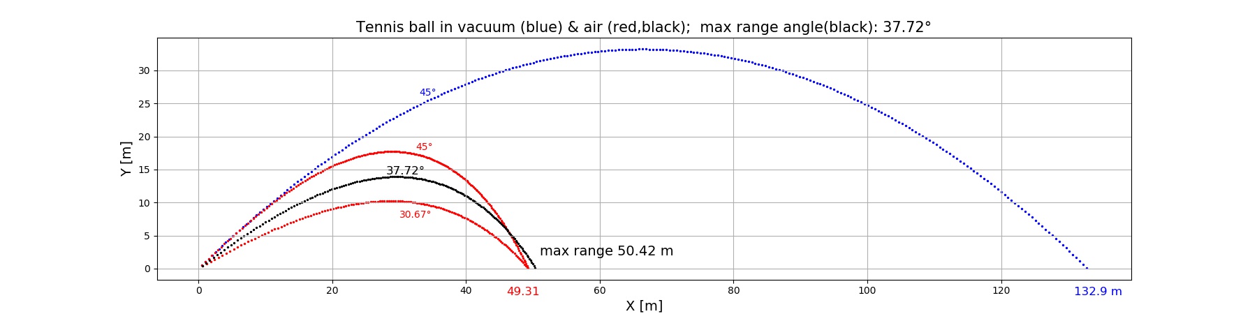
With the tested procedure, find the angle $\alpha_m$ which results in maximum range $R$. What are the quantities (i)-(iii) then? Plots of trajectories are welcome!

Solution

Notice how little the range changes for a wide range of launch angles (30-45 degrees), only by 1.11 m on a distance of 50 m.

Python code.
The script uses the simplest method possible (1st/2nd order accuracy with a short timestep dt=0.001 s). Notice that high-rder methods are not needed in view of the short running time. However, there is one thing which can make the code very slow: graphics done during calculation. If, in order to save RAM points on trajectory are not stored in arrays, and instead every computed point is immediately plotted using pyplot.scatter(x,y) command, then the runtime is long. In the above program, one every 20th point is plotted. This assures but is not motivated by saving running time. It is done to visually indicate the speed along trajectories (via visible point spacing).

Times of travel were not part of the exercise & are not plotted, but they are trivial to print out. They differ a lot, as do maximum heights H:
T (vac, $\alpha = 45^\circ$) = 5.295 s,   range = 132.9 m, max H = 33.21 m
T (air, $\alpha = 45^\circ$) = 3.766 s,   range = 49.31 m, max H = 17.72 m
T (air, $\alpha = 37.72^\circ$) = 3.330 s,   range = 50.42 m, max H = 13.90 m
T (air, $\alpha = 30.67^\circ$) = 2.856 s,   range = 49.31 m, max H = 10.21 m

As to the asymmetry factor (0.500 in vacuum), in air it is constant to within 1% ($x_m/R = 0.588, 0.587, 0.583$) in the three cases shown above.

Problem 1.2 [22 pts] Maximum unidirectional drop of value

You are given a series of values $x$ of length $N$; that is a vector of values $x_i$, where $i=1...N$. Formulate an algorithm that finds the maximum drawdown (maximum drop) of $x$ (representing investment or voltage) in some contiguous segment of data, i.e. the largest drop of value from some initial value $x_i$ to a lower value $x_j$ at index $j > i$.

For instance, if the series is $x$ = {4, 3, 6, 5, 4, 5, 2, 3, 4, 4, 11, 8, 10} then the largest dropdown is between positions $i=3$ and $j=7$, and equals $x_3-x_7= 6-2=4$. Notice that we could have even more points between those two, with values oscillating between 2 and 6, and the resuting maxmium dropdown would not change. A different $j$ might result but we are not interested in $i$ or $j$, just the maximum drop (precise interval can be provided with very little extra work, but the problem does not ask for it). Your algorithm must thus somehow not be fooled by local extrema.

You can describe your algorithm in words, and/or implement it, commenting the program very well, so it is clear how it works and how you proved that it correctly works to yourself.

Remark: Since all contiguous subsets (subintervals) of the dataset provide possible solution, examining them all separately would take an effort of computational complexity $O(N^2)$, because the number of all index pairs {$j\gt i$} is $N(N-1)/2$, so $\sim N^2$. For large $N$ this is an awful lot of computation. Try to obtain a cheaper asymptotic scaling with $N$ if you can. If you can't, code an inefficient method scaling like $N^2$, for a partial credit of up to 13 pts.

Solution

One needs only to change the maximum to minimum, or leave the maximum and just reverse the sign of all the data.

The problem has an $O(N)$ solution, much faster than the simplest $O(N^3)$ solution consisting in checking all contiguous subintervals of a 1-D set of numbers. [Yes, it's that bad, if you use series of differences, because there are of order $O(N^2)$ subintervals, and each requires of order $O(N)$ additions to do the sum within subinterval.]

Every time-series or a 1-D spatial scan of physical variables can be easily differentiated numerically, i.e. turned into a series of next-neighbour differences of values. That transformation preserves information in the same amount of RAM (N-1 differences plus 1 starting value of the original series = N values).

def max_subarray(numbers):
    """Find the largest sum of any contiguous subarray."""
    best_sum = float('-inf')
    current_sum = 0
    for x in numbers:
        current_sum = max(x, current_sum + x)
        best_sum = max(best_sum, current_sum)
    return best_sum

How the algorithm for our problem works can be described like this. Think of money in an investment account as a function of discrete time, $X(t_n)$ or $X_n$. The task is to find a contiguous subinterval with the biggest drop of account holdings. You start at the beginning of data and assume for a while that this is where the optimal subinterval begins. Remember in some variable the starting value, you can call it $x_0$. If the holdings initially drop, you continue, wait to see how big a drop you can record. You track the biggest drop encountered so far, i.e. $\Delta = \min (X_n - x_0)$. The values of $X$ will sometimes reverse and go up for a while, fluctuate up and down, but you ignore these local extrema, with one notable exception.
When you encounter a value $X_n$ which is higher than $x_0$, well that may change the situation! It gives you a chance of recording (later) a bigger drop from that higher peak, if the values go low enough, which is not known in this single pass through the data -- but you must act nevertheless. Overwrite $x_0$ with a higher $X_n$, and continue counting $\Delta$'s with the updated $x_0$. You also store somewhere (say, in variable $\Delta_{best}$) the best (most negative) $\Delta$ encountered so far, just in case you actually can't find any better $\Delta$ in the rest of the data. In the end, you scannned the data just once, $O(N)$ work.

I also liked the idea of one of you - in the worst case it is still almost as inefficient as the simplest one, but in practice it is much faster than literally finding all subintervals of length $N$ data; the method typically will have a much better coefficient in front of $N^2$. You first scan the data in $O(N)$ time and forget all individual data, except the local extrema. This typically reduced $N$ considerably! Paradoxically, focusing on, instead of ignoring, local extrema already should help. How much? Depends on how choppy the series is! If it's very noisy, the speedup will be so-so, but for smoother data, it will be a big help.

Problem 1.3 [15 pts] Second order stencil for curvature

Show it numerically for a particular choice of function: $$ y(x) = e^{x-1} + x^3(x - 1) $$ around the point $x=1$. Make a plot of the difference between true analytical second derivative and its estimate $f$ above, as a function of $h$.

The plot should have a log-log scaling to reveal any power-law dependencies between the error and $h$. (What is the slope?) The suggested range of $h$ should be from, say, $10^{-7}$, to $10^{-2}$. and the power of ten that produces $h$ (not $h$ itself) should cover that range uniformly. Otherwise there will be a pileup of points toward one end of the plot in log-log axes.

Solution

Substitution into the $f(x,h) = ...\;$ formula yields: $$ f(x,h) = y^"(x) + y^{""}(x) \,h^2/12 \;+\;...$$ which proves that the inaccuracy is $O(h^2)$, making the scheme 2nd order, as advertised.
The log-log plot of $|f(x,h)-y^"(x)|$ vs. $h$ should show the slope of +2, i.e. error decreasing with decreasing spacing $h$ as $h^2$, down to a point where the accuracy of additions and subtractions reaches the arithmetic roundoff limit. After that, further decrease of $h$ only increases the error because the denominator is $h^2$ and quickly decreases as $h$ decreases. Estimator will then show $\sim h^{-2}$ scaling and can produce horrible errors for very small $h$. Let's see where the change of behavior of abs(error) happens, and what is the best $h=h_{opt}$ and the smallest possible error of $f$.

The error of the numerator of our approximator of $y^"$ cannot be smaller than one or a few machine epsilons or minimum representatable real/float values. Assume optimistically $\epsilon \approx 10^{-16}$. Since the denominator is $h^2$, our estimator's minimum error is $O(10^{-16}/h^2)$. We don't yet know at which $h$ that happens. From Taylor expansion of our function around $x=1$, the numerator's error $\approx y^{""}(x) \,h^2/12$, which (given that the 4th derivative evaluates to 25 at $x=1$) evaluates to $(25/12)h^2$. Equating this with $\epsilon$, we obtain $h_{opt}\approx 10^{-4}$, and the minimum estimator's error $O(10^{-16}/10^{2(-4)}) = O(10^{-8})$.

One of the possible numerical programs in python is in the phyd57 account on art-1:

 ~/prog57/y_xx.py 

Some of the difficulties with this assignment that I noticed involved not giving enough thought to the results. If the error does not appear to change with $h$, or changes in the wrong direction (estimate of curvature gets more inaccurate with decreasing $h$, for most values of $h$) - then something's wrong and the result does not warrant a submission to Quercus.

Problem 1.4 [15 pts] What are the FPGAs and ASICs?