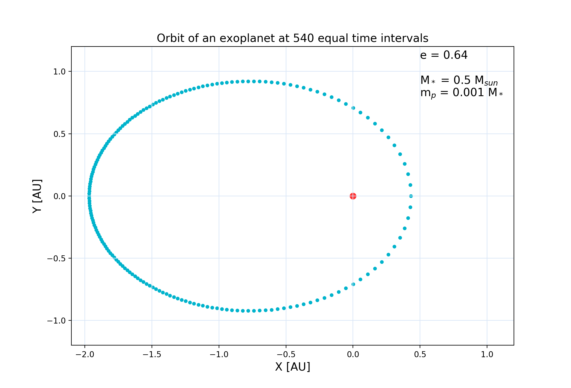
An ellipse in polar coordinate system, where $r$ will denote the instantaneous distance between the 2 bodies, can be written down as a function of either $f$ (the so-called true anomaly, angle between the vector drawn from the focus to the object travelling on ellipse, and the line of apsides, which by definition joins the periastron and apoastron, i.e. the closest and the furthest points of the orbit), or of another angle $E$ called eccentric anomaly: $$r(f) = \frac{a(1-e^2)}{1 + e\,\cos f} = r(E) = a(1 - e\,\cos E)\,,$$ where $e$ = nondimensional eccentricity parameter describing the shape of the ellipse, $0 \le e \lt 1$. For illustration of an ellipse, see wiki article on elliptic orbits. Both angles $f$ and $E$ change in time, starting at value zero at pericenter (closest approach time) up to $2\pi$ radians, back at the pericenter again. They are interependent: $$ \tan \frac{f}{2} = \sqrt{\frac{1+e}{1-e}} \; \tan \frac{E}{2}\; $$ In elliptic motion, angle $f$ depends on time in a complicated way that we don't know directly. We get $f(t)$ via $E(t)$, ever since Johannes Kepler proved that planet's paths are elliptical and provided us with the following equation for $E$ (but not directly for $f$), called Kepler's equation: $$nt = E - e\, \sin E.$$ In it, $n$ denotes the mean angular speed of the system (this constant in some applications is called $\Omega$ but in astronomy it's better to stick to the historical use of $n$, because an unrelated $\Omega$ that is a certain positional angle not an angular speed, comes up). For example, Earth-sun system would have $n = 360^\circ$/yr. The product $nt$ is an angle called mean anomaly. Mean anomaly is the positional angle when $e=0$ and $f=E=nt$. Likewise, it is uniformly growing in time even when $e>0$.
Over one hundred numerical methods have been tried since the times of J. Kepler to quickly solve his transcendental equation for $E(t)$, or more precisely, $E(nt)$. When eccentricity isn't very close to unity, the equation can be solved by iteration. $E_n$, the $n-$th approximation of $E$, is obtained from $E_{n-1}$ like so (as folows from Kepler's eq.): $$E_n = nt + e\,\sin E_{n-1}\,,$$ with starting value $E_0 = nt$, until the value of $E$ practically stops changing (the absolute value of change of $E$ from one iteration to the next becomes less than, say, 1e-9). To be safe, also hard-code the number of iterations to be 40, should the criterion not work correctly (causing an infinite loop).
Every $t$ requires a separate iterative solution of Kepler equation. Once $E(t)$ and then $f(t)$ is found, you can plug either one into the above equations of ellipse. This is, by the way, described in wiki pages on eccentric anomaly and Kepler equation.
Let's begin the velocity components calculation from the motion perpendicular to radius (radial direction), at linear speed $v_\perp = r \dot{f}$ and angular speed $\dot{f} = df/dt$. Expression $L = r^2\,df/dt = r v_\perp$ is a constant specific angular momentum, $L = \sqrt{GMa(1-e^2)} = const.$, so we can also write $v_\perp = L/r$ at any time.
Now, what is the radial velocity component $\dot{r} = dr/dt$? One easy way of obtaining it when one knows $E$ and/or $f$, is taking full time derivative of the expression of $r(E)$ or $r(f)$, not forgetting the inner derivative $dE/dt$ or $df/dt$, correspondingly. These derivatives can be written down looking at either the Kepler's equation or the $L$-conservation principle. Do it your preferred way.
So far we know how to obtain velocity components $v_\perp$ and $v_r$ of the relative orbit of the planet around star. The motion of the star is a reflex motion and by assumption 180 degrees out of phase and smaller by the planet:star mass ratio (both the distance vector and the velocity components get multiplied by $-m_p/(m_*+m_p) = -m_p/M$. If we were seeking the position and velocity components of the planet, we would use a factor $+m_*/(m_*+m_p) = m_p/M$ to multiply the relative orbit; the two factors must sum up to 1 in absolute value. For instance, if the planet moves at 30 km/s (in any direction, in the frame of the center of their mass), then the star moves at -30 m/s, if the planet is 103 times less massive than the star.
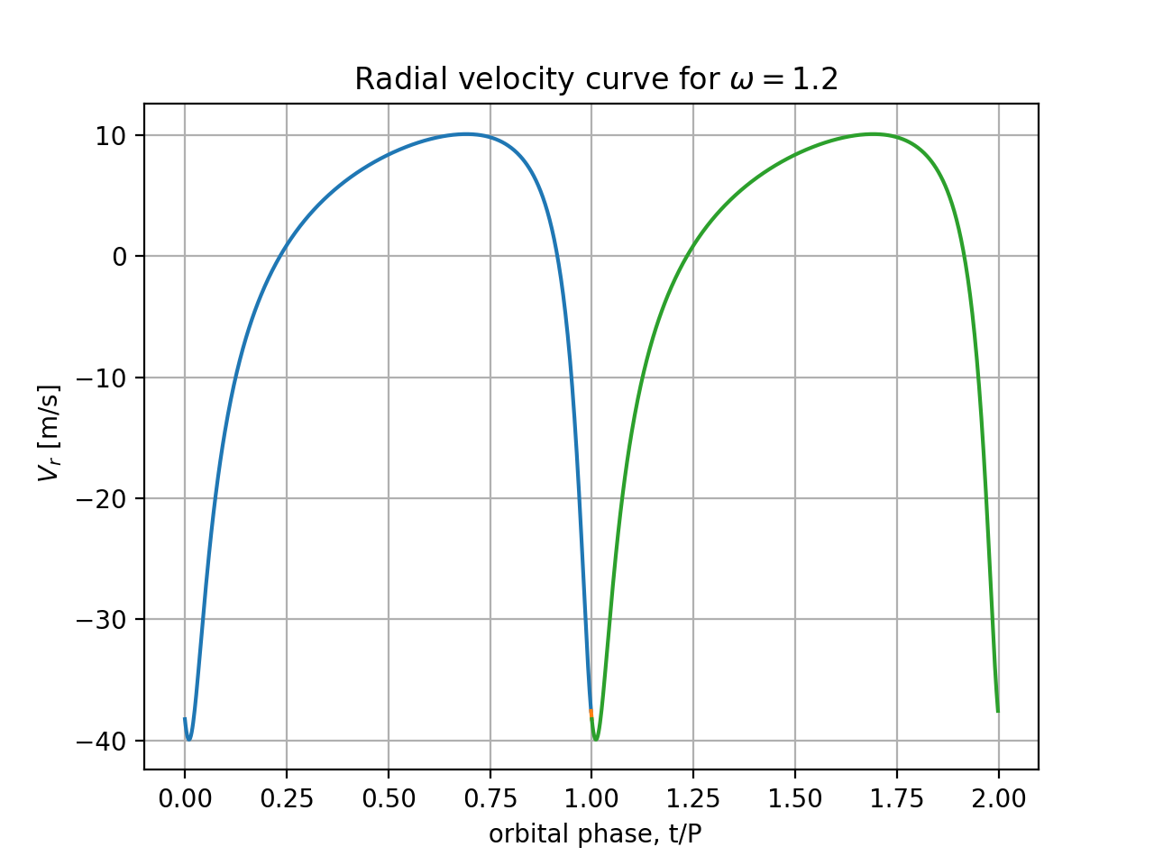
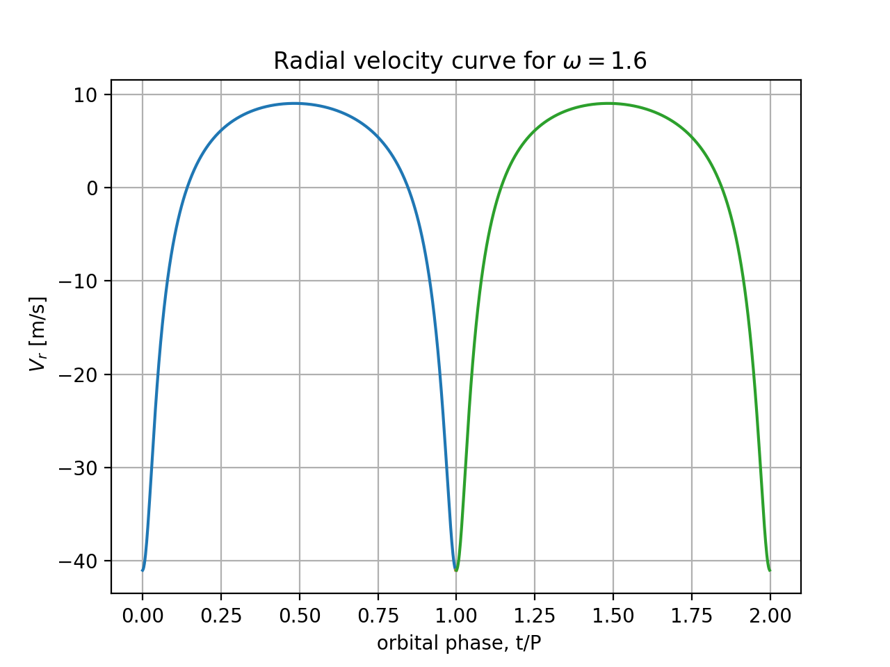
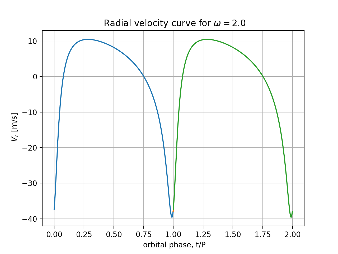
By projecting the star's velocity onto the line-of-sight, verify whether the line-of-sight component of velocity in elliptic motion, which we as distant observers call radial velocity (using line-of-sight as radial direction) equals $$ V_r = -\frac{m_p}{M}\; \sqrt{\frac{GM}{a(1-e^2)}} \;\;[\sin(w+f) (1+e\,\cos f)-e\,\sin(f)\;\cos(w+f)]$$
I believe this is correct, but your task is to check everything. Submit and use your formula with derivation. A fact useful for coding: $\sqrt{GM_\odot/1 \mbox{AU}} = 29.78$ km/s.
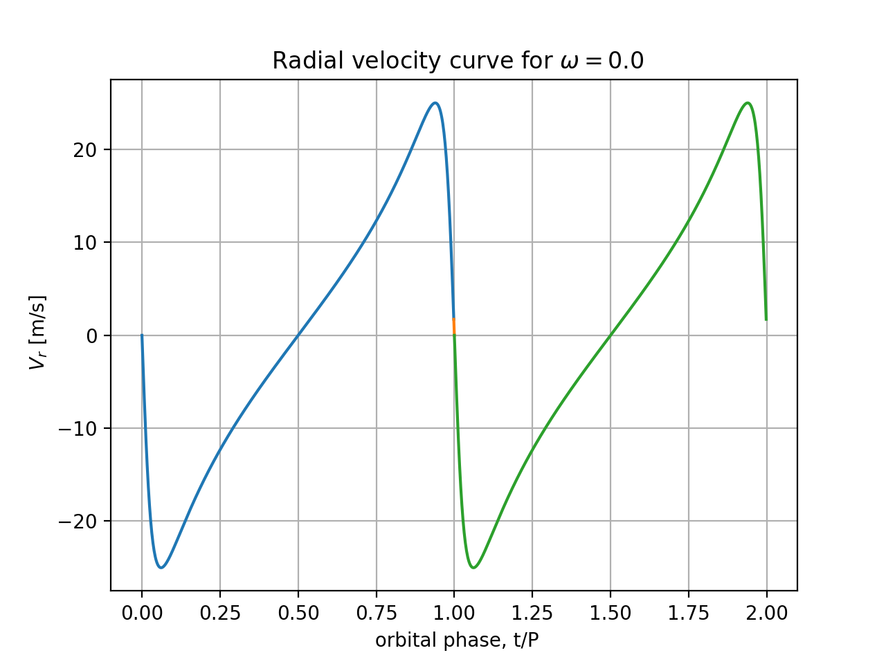
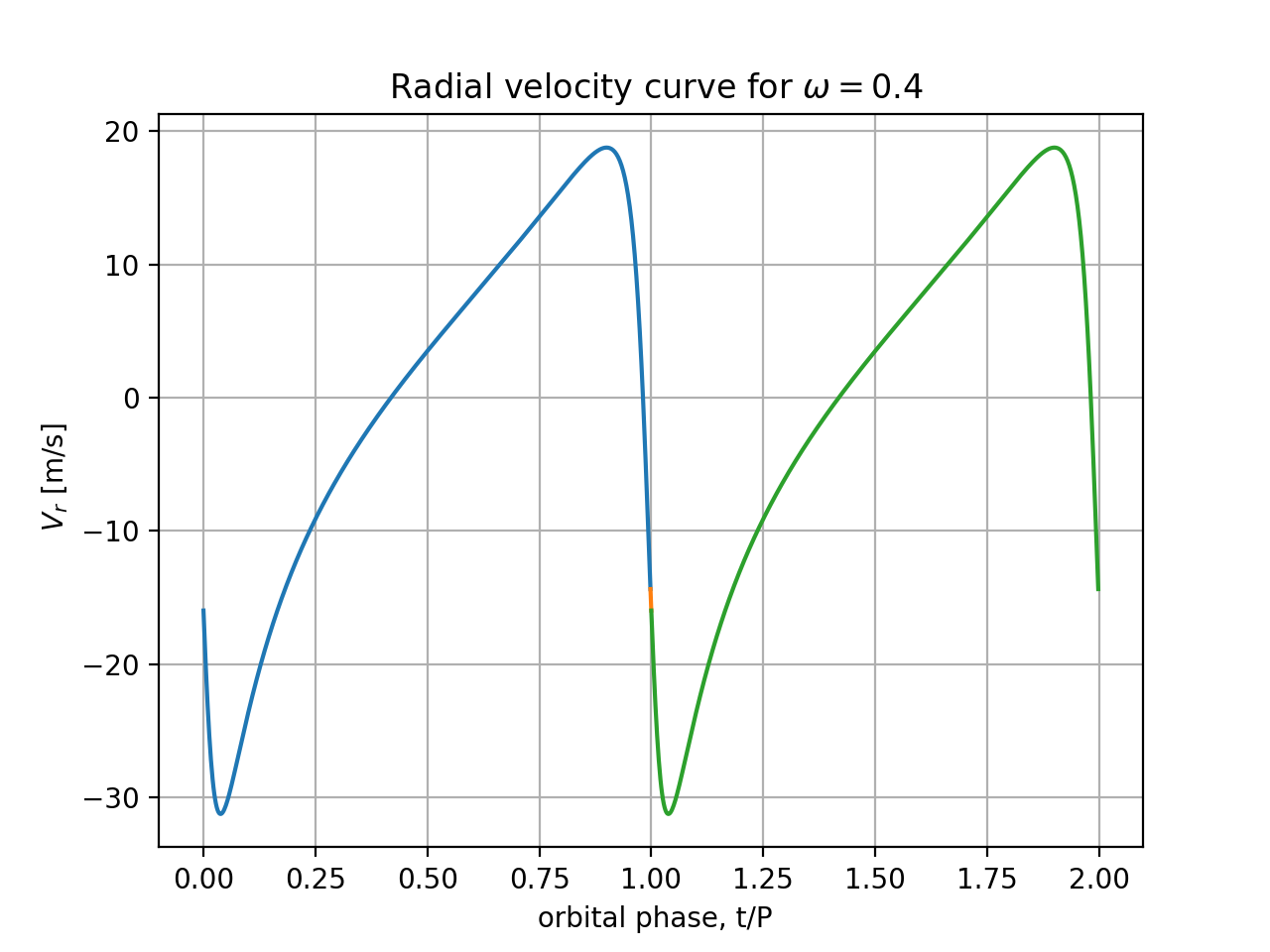
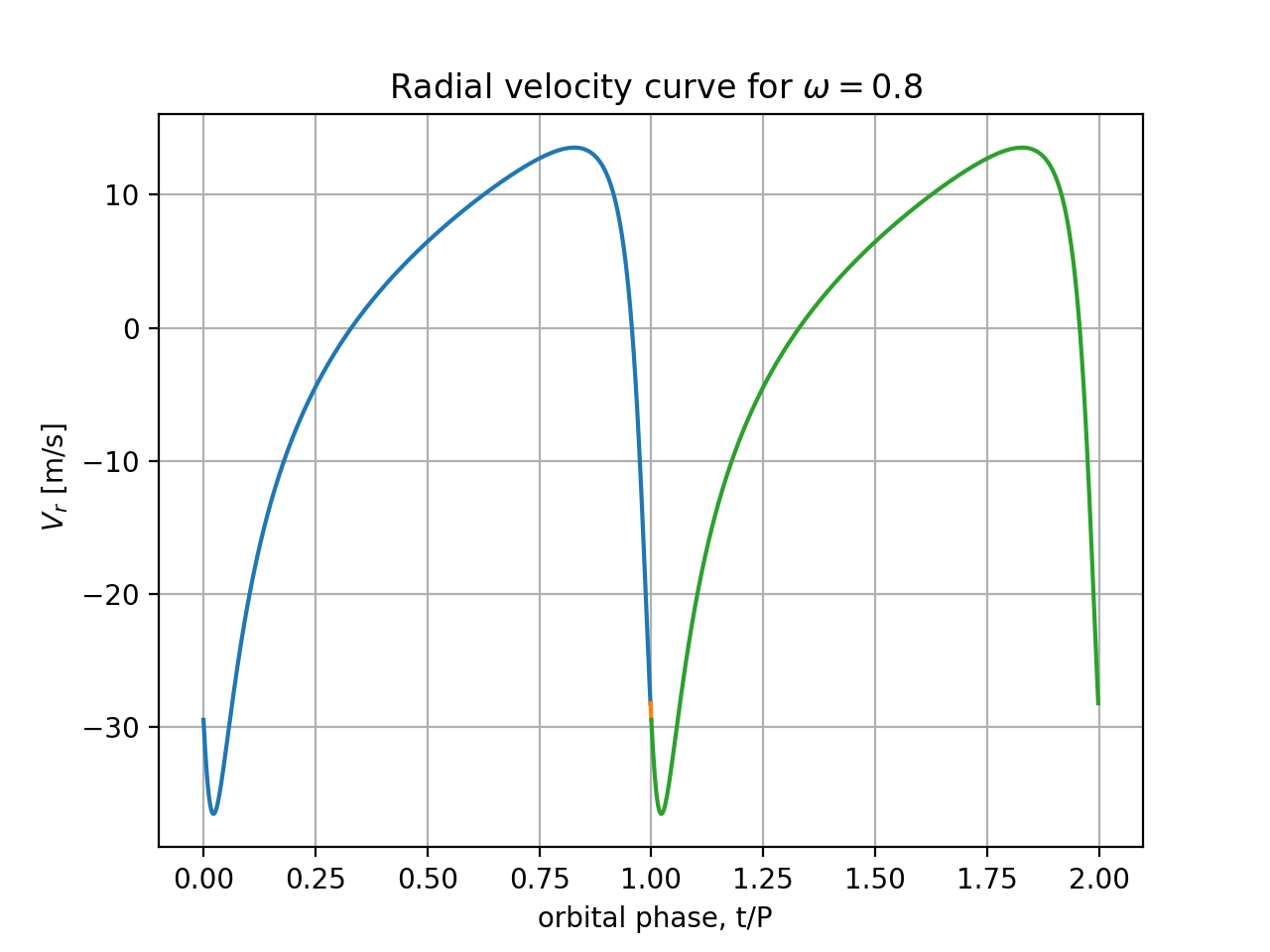
Plot
$V_r(t)$ for $M=0.5 M_\odot$, $a=1.20$ AU, and $e=0.64$, $m_p/M=0.001$,
for 2 choices of orientation angle:
$\omega=0$ and $\omega= 2$ rad. You can overplot the 2 radial velocity
curves in one figure. Make sure labels and values under axes are
present and clearly visible, labels and units of variables are correct.
Plot a range of phase angles $nt = 0...10$ radians (use $nt$ as horizonal
plot axis), i.e. almost two full periods of motion. Plot curves
of N=400 or more points, uniformly spread between extremes of time/phase.
Is the full amplitude of the velocity curve (maximum minus minimum values) independent of $\omega$? Please explain why the shapes are different and in neither case resemble a sinusoid.
Although it's up to you, you may want to develop your code bottom-up, first writing a tiny driver main program that states some sample values of parameters and tests the Kepler-equation solver. Once you test that function by inserting some print or printf instructions and seeing the correct output for sample iterations, comment out the printing, since it is no longer needed and just takes a lot of cpu time. Then write a wrapper routine using the Kepler-solver to produce two velocity components for one input value of $nt$. After successful testing, write a higher-level routine that uses those velocity components or implements the $V_r$ formula directly, and covers a whole range of times. Plotting routine will just use the computed values.
They release them at time t=0. Particles have electric charge opposite to electron charge. Gravity and other forces can be neglected. Show that because of the symmetry, particles trace semi-infinite straight lines along the diagonals of the square. Find particle trajectories numerically, as distance from square's center vs. time at t > 0. Use symmetries to reduce the amount of work, maybe not all four particles need to be followed. Is the total energy conserved? It's also a sort of symmetry. Use it. At $t\to \infty$, find the ratio of positron to proton speeds, and the ratio of their kinetic energies. If the temperature scales with the mean kinetic energy per particle according to $kT = \lt m v^2/2 \gt$ ($k$ being the Boltzmann constant) then what are the values and the ratio of the 'temperatures' of positron and proton energies at infinity (quotations mark are here to remind of very small statistics, such that the thermodynamical concept of temperature as am average does not apply.
Use Fortran or C. Comment the codes thoroughly. Monitor the accuracy by tracking the total energy E (kinetic and potential energy of the system) and printing from time to time during the calculation the relative error in energy dE/E0 = (E-E0)/E0, where E0 = E(t=0). Either vary timestep of your integration scheme as a function of distance between particles, or keep it constant for simplicity, but assure (and describe) a reasonably good accuracy of total energy conservation. Integration scheme is up to you; give the motivation for your choice.
Compare your answer with the simplified analytical solution done with paper and pencil as follows. Assume that protons, being much more massive (find the physical laws and constants on wikipedia), move so slowly compared with the lighter positrons, that the latter actually 'think' that protons are always at rest, while protons 'think' that electrons have escaped instantaneously, before protons had a chance to move much from rest. Assume energy conservation law for e+ and p+ particles separately in the analytical calculation.
Hint: The given value of d is unimportant for the shape of trajectories and the asymptotic ratio of v_e+ / v_p+. Can you convince yourself of that? How can you simplify the equations to reflect this: do you really need all the physical constants in correct SI units in the equations? Do you need x and y coordinates or just one along the trajectory? Maybe it is enough to solve for the motion of two types of masses with the correct mass ratio, starting at (square side) distance = 1, under force law F = +1/r^2 between the particles, and of course using the diagonal symmetry. If you're not convinced, solve the problem the hard way first, with dimensional constants, precise laws of electrostatics etc.
Accelerations of protons and positrons ($f_x$ and $f_y$) are (-1/2) times the derivatives of $U$ along the trajectories, divided by appropriate mass: $$ \ddot{x} = f_x = \frac{q^2}{4 \pi \epsilon_0 m_e}\,\left[\frac{1}{4x^2} +\frac{2x}{(x^2+y^2)^{3/2}}\right] $$ $$ \ddot{y} = f_y = \frac{q^2}{4 \pi \epsilon_0 m_p}\,\left[\frac{1}{4y^2} +\frac{2y}{(x^2+y^2)^{3/2}}\right]$$ These are two coupled 2nd order ODEs to be numerically integrated forward in time.
The simplified model
..assumes that protons hardly move at all during the acceleration of positrons, so $y=y_0=const$ can be assumed during the evolution of $x$. For protons, we can but don't necessarily have to assume that the light particles immediately depart to infinity, because during their quick departure they still can impart some momentum to protons. Why don't we leave that issue for later and solve the motion of lighter particles first. (Maybe we can get some extra precision by inclusion of known approximate motion of positrons, if we gain enough insight.) In any case, stationary protons assumption implies that protons gain of energy is unimportant; all or almost all the initial electrostatic energy should end up in positrons. The validity of that assumption we'll have to verify at the end of the simplified calculation.
Using the energy conservation principle $E_0 = U + m_e\dot{x}^2/2$,
where $E_0 = U(t=0)$, and electrostatic energy $U$ contains $y=y_0=const$,
our simplified model leads to
$$ \dot{x}^2 = \frac{2(E_0-U)}{m_e} = \frac{q^2}{\pi m_e \epsilon_0}
\left[\frac{1}{4x_0}-\frac{1}{4x}+\frac{2}{\sqrt{x_0^2+y_0^2}}
-\frac{2}{\sqrt{x^2+y_0^2}} \right]$$
Separation of variables gives
$$ t = \int dt = \frac{\sqrt{\pi m_e \epsilon_0}}{q}\,\int^x_{x_0}
\left[\frac{1}{4x_0}-\frac{1}{4x}+\frac{2}{\sqrt{x_0^2+y_0^2}}
-\frac{2}{\sqrt{x^2+y_0^2}} \right]^{-1/2}\, dx $$
but the integral is difficult to evaluate analytically, so we won't try
to obtain a nice analytical formula for $t(x)$, and then invert it into an
explicit formula for $x(t)$.
Instead, let's just extract the asymptotic information from the $\dot{x}^2$
formula above:
$$\dot{x}_\infty = \frac{q}{\sqrt{\pi m_e \epsilon_0}}
\left[\frac{1}{4x_0} +\frac{2}{\sqrt{x_0^2+y_0^2}}\right]^{1/2}.$$
We got what we easily could derive about positrons.
Now turn to protons. Assuming that the lighter particles are long gone during the proton acceleration, except for a very short period of time when positrons are still close by (so short that not much $p^+$ momentum builds up due to $p^+-e^+$ interaction), we will entirely neglect positrons and solve a 2-proton problem (subbing $x\to \infty$ into the energy formula). Conversion of $U_0 = q^2/(8\pi \epsilon_0 y_0)$ into kinetic energy would give protons the asymptotic speed $$ \dot{y}_\infty = \frac{q}{2\sqrt{\pi m_p \epsilon_0 y_0}}.$$ Finally, we apply the initial configuration of 4 particles in a square with side $a = 100$ fm, which implies $x_0=y_0 =a/\sqrt{2}$, to simplify the obtained speeds at infinity to $$ \dot{x}_\infty = \frac{q}{\sqrt{\pi m_e \epsilon_0 a}} (2+\sqrt{2}/4)^{1/2};\;\;\;\;\; \dot{y}_\infty = \frac{q}{2^{3/4} \sqrt{\pi m_p \epsilon_0 a}}.$$ The ratio of speeds at infinity is equal $$\frac{\dot{x}_\infty}{\dot{y}_\infty} = \sqrt{\frac{m_p}{m_e}\; (1+4\sqrt{2})} = 110.58 $$ where we have used $m_p/m_e = 1837$. The ratio of kinetic temperatures, or simply kinetic energies at infinity, is $$\frac{E_{kin, e^+}}{E_{kin,p^+}} = \frac{m_e\dot{x}_\infty^2 } {m_p\dot{y}_\infty^2}= 1+4\sqrt{2}=6.6569\,.$$
For comparison, an ideal energy equipartition (that is, $E_{e^+}/E_{p^+} = 1$) would mean $$\frac{\dot{x}_\infty}{\dot{y}_\infty} = \sqrt{\frac{m_p}{m_e}} = 42.86$$
By substitution of physical constants, you can
calculate individual final speeds of particles in m/s, you can also convert
them to temperatures in kelvins. It turns out that electrons would
gain on the order of 1/3 the speed of light, and become almost relativistic.
Conversion to temperature (which we call kinetic temperature,
because the particles themselves are not 'hot' in any sense, if they
hit a wall then maybe the wall would get locally hot!)
can be obtained from
$$kT/2= m v^2/2$$
The l.h.s. is the thermal energy in one direction,
here given by the direction of motion of particles.
You would thus get a 6.657 times higher temperature $T$ of anti-electrons.
So which way were your numerical calculations pointing? Which theory is better, equipartition or our approximate scenario?
My numerical results:
I took a very small timestep for accuracy, and let the particles go far
from the initial square: the protons coasted to 660*100fm, travelling
only about $10^{-3}$ fm per timestep on average. Positrons departed 110.9
times further, doing at most $\sim 0.1$ fm per step.
The computed final positron:proton speed ratio was 110.56, which differs
from the analytical estimate by only 0.02%. The kinetic temperature T
(kinetic energy) ratio was 6.6537, which differs from $1+4\sqrt{2}$
only by 0.05%. Thus, the immobile-proton-mobile-positron approximation
turned out extremely accurate, while the equipartition theory is off
by an order of magnitude, predicting ratio of temperatures of 1.0000.
My numerical script was simple & didn't output any S.I. values of
speeds or temperatures, just their ratios. It looked like this:
pepe.py , and took a long time (a minute) to complete, since
it's in Python. Yours should finish much quicker.
I am actually solving equations that look like
$$ z = 2/(x\,x+y\,y)^{3/2}$$
$$ x^" =1837 (0.25/x/x +z\, x) $$
$$ y^" =0.25/y/y +z\, y, $$
instead of the full pair of ($\ddot{x}, \ddot{y}$) equations shown above.
It's called non-dimensionalization, the units of time and distance have been
changed to more natural ones for the problem. Not only does this (i)
speed up the calculation (fewer arithmetic ops!), but also (ii)
makes it more generally applicable after just one integration.
The solution is trivially rescaleable to any values of constants,
like the initial distances of particles (still in
a square), different (but still equal) electrical charges, even parallel
universes with alternative dielectric vacuum constant $\epsilon_0$. Don't ask
if we could have a differing value of $\pi$ there. Maybe. I'd miss our
"Yes I need a drink. Alcoholic of course, after the heavy
lectures involving QM" $\pi$. Make sure you understand why time unit
in my code is what the comments in the code says, especially if you want
to understand the units of speed and convert it to temperature in kelvins.
Incidentally, this mnemonic for $\pi$ shows you why ASCII coding is
inefficient. How many letters are in the sentence in the quotation marks,
how many decimal digits in $\pi$, and how many bytes needed to store each
representation, compared with just 8 bytes for double precision binary
representation? If memory is a limitation, heavy duty calculations should
store data in binary format, not in ASCII. HPC languages allow that.
Finally, there is (iii) the 3rd reason to consider rescaling equations. Values of variables are not as extreme as they get in some problems, this one being a good example. This prevents accidentally exceeding the range of exponents in floating point arithmetic. Some of you reportedly took the idea of how to set the timestep dt from other calculations, where staring distances and forces are not far from 1 in value. Then dt=0.01 or (just to be sure) dt=0.001 could work. But if you stick with the S.I. units, dt cannot be 0.001 seconds. It should be dt $\lt 10^{-23}$ s, 10000000000000000000x smaller. If particles are a few times 100 fm apart, you want them to be pushed by less than 1 fm in each timestep, right? But electrons get dangerously close to be relativistic, i.e. travel at about 1e8 m/s, so dt $<$ 1 fm/(1e8 m/s) ~ 1e-23 s.
I think many of you obtained speed ratio at
infinity close to mass ratio $m_p/m_e = 1837$. That's wrong, because
it should be about 111, and a rough guess would be $\sqrt{1837}$
from equipartition. This mistake is because incorrect speeds are given
to the particles in the first (and the only important!) timestep.
They are dt*acceleration, hence differ by factor $m_p/m_e$. Namely,
all the forces are equal in initial configuration, and acceleration
is force/mass. In later timesteps, particles are unrealistically far
& don't really interact, so they don't change their speed much.
But a wrong dt violates energy conservation, which
you ahould have easily detect!
Remember to always use integrals of motion in dynamical calculations
as diagnostic tools of the quality of numerical precision.
Print out the relative change in, e.g., energy (not
the absolute value of increase, since often absolute values are not
familiar and can mislead.)
A. What is the probability that the two arrivals on a given day are separated by less than 1/3 day?
Hint: Look at the event space as a square in coordinates $t_1$ and $t_2$ (the arrival times of particle 1 and 2). Alternatively, redefine those variables and consider the upper-triangular half of that square, i.e. name the earlier arrival time $t_1$ and the later time $t_2$.
B. Theoretically calculate the following average time intervals:
(i) before the arrival of the first particle, (ii) between their arrivals, (iii)
after the second arrival.
Hint: Average should be done over the appropriate areas in the $t_1, t_2$ plane.
Quantity $X(t_1,t_2)$ averages out to
$$ \braket{X} = \frac{\int \int \, X(t_1,t_2)\; dt_1\, dt_2}
{\int \int dt_1 \, dt_2 } $$
where the area of double integration is either a square or a triangle, as mentioned
in point A. The denominator assures proper normalization, namely the average
of a constant $X$ must be $X$ itself.
C. Compute numerically tasks A and B by MtCarlo method (pseudo-random number
generation, see hint 1 below).
Study $N=10^8$ samples. As the calculation proceeds, print its results
after accumulating the averages/probabilities over $N=10^a$, where
$a = 2,3,...8$.
The result should include the standard deviation (see hint 2 below).
Example below uses fake numbers, and assumes that $t_1 < t_2$:
(...)
N = 10000, t1 = 0.417 +- 0.012, t2-t1
= 0.311 +- 0.023, 1-t2 = 0.282 +- 0.034
(...).
Discuss the results thoroughly. Compare sections A and B. Study the rate at which MtC converges to analytical or asymptotic numerical results as $N$ increases. Formulate an empirical, upper bound, powel-law formula for relative error in this problem, as a function of $N$, for large $N$.
Hint 1: For a simple MtC method and random numer generation, cf. simple-mtc.f90 on our coding page: page , program . Or find the syntax of a standard random numer generator in C++ compiler guide cited on the hidden page.
Hint 2: Variance $\sigma^2$ = square of standard deviation.
Let brackets $\braket{y}$ denote averaging of arbitrary quantity $y$.
From the definition, the variance of $y$ equals
$$\sigma_y^2 = \braket{(y - \braket{y})^2} =\braket{y^2}- \braket
{2 \braket{y} y} + \braket{y}^2 =\braket{y^2} -2 \braket{y}^2 +
\braket{y}^2 =\braket{y^2} -\braket{y}^2.$$
The last form allows you to avoid doing two separate passes through
your data set, one to find arithmetic average $\braket{y}$, and the
second to find $\sigma_y = \sqrt{\braket{(y- \braket{y})^2}}$.
In this particular problem, for instance, there is no need to store all
the generated pairs of random numbers.
One can evaluate both $\braket{y}$ and $\braket{y^2}$ in the same single
loop that generates the random numbers,
by introducing variables holding 2 partial sums. After summation,
don't forget to divide the sum by the number of the summed items.
Think about the meaning of sigma. In literature, it may mean standard deviation
of values around their mean, or the standard deviation of the mean value.
They different a lot, by a factor $\sqrt{N-1}$, as explained in file
simple_stat.py on our code page.
If you are interested in mathematical approximations known as "law of planetary distances" in the 18th-20th cent., and now just as "rules", see wiki on Titius law. Especially simple is the form proposed by Mary Blagg more than a century ago. Planets in our Solar System are at mean distances from the sun (semi-major axes $a$, to be more precise) that seem to follow a curiously regular spacing rule, expressing the distance of planet number $n$, i.e. $a(n)$, as a simple function of $n$. Here is the Blagg form: $$ a(n) = x^n. $$ Simple, isn't it? $a(n)$ is in astronomical units (AU), and $n$ is the number given to the 9 bodies of the system in the following way: -2,-1,0,1,...6 correspond to: Mercury(-2), Venus(-1), Earth(0), Mars(1), Ceres(2) - it's the largest asteroid in the main belt, Jupiter(3), Saturn(4), Uranus(5), and Neptune(6). Obviously, some more distant and more recently discovered bodies are omitted for historical reasons and, truth to be told, they don't obey the rule so closely, that's why we call such formulae rules not laws.
Write a code where you declare and fill a small, flating point, 1-d array of the semi-major axes (in AU) called "a", of all 9 bodies. Find the $a$ values with 3 accurate digits somewhere, e.g. in wikipedia. This array will not change in the beginnig.
Another, 1-D integer array will be called "n", and will contain the integer labels from -2 to 6. Those are all the inputs that we need. The trial prediction of the distances, named "d" (and measured in AU), will be a vector (1-D array) of length 9.
[Although d = x**n is meta-code, this happens to be precisely how we compute $d$ in Fortran and Python, based on the curent value of x. Notice that in C you cannot use a one-liner like d = x**n, you have to explicitly write a loop from 1 to 9, using a constant value of $x$ and the loop index $n$.]
Now it remains to minimize the deviations between predictions and reality somehow. The optimum value of parameter $x$ is unknown, it will be found by fitting theory ($d = x^n$) to the data ($a$). Vector of deviations between theory and observation will be ($d$-$a$) and, more importantly, we won't be interested in it. Rather, we use the length-9, relative error vector $\Delta = (d-a)/a $ normalized by observed values.
Let us minimize $E$, the quadratic sum of
the relative errors of the prediction contained in array $d$:
$$E = \sum_{i=1}^9 [(d_i-a_i)/a_i]^2 \to \min$$
It's the average, relative, quadratic error, except that
we skip dividing the sum by 9 (why bother?).
Write a function for E(x). In Fortran it may look like a one-liner
E = sum((d/a-1.)**2), similarly in Numpy it would be
np.sum((d/a-1.)**2), or much less compact instructions in C(++).
Notice that you minimize the sum of squares of the relative, not of
the absolute, deviations of theory from observations, which would be coded
without the division by "a".
For some $x$, probably between $x=1.5$ and $x=2.5$, lies the best fit to observational data, producing a minimum error E. Compute the best-fit $x$ as an automatic root finding problem, using bisection method (cf. PHYB57, Turner et al. textbook) on $dE/dx$ (differentiate analytically the expression for $E$, and write a function to evaluate the derivative or 1/2 of it, whichever computes faster, making sure the signs of it differ at the beginnig left and right x-boundaries). Or use any other method you like to minimize $E$ directly. As always, (i) write your original code throughout, don't use internet, AI or specialized Python modules. To understand how it's done, you have to program it yourself; (ii) explain what you did throughly, and put comment lines in the code, among others to show that you wrote the thing.
A. What is the optimum $x$?
B. Can you estimate the uncertainty of this parameter of the model? Think of changes to $x$ that would cause a noticeable increase of $E$, or think of artificially disturbing the observational data within tolerable limits (creating a cloud of artifical datasets) consistent with observational uncertainty, and then letting the program do the fitting to all datasets separately, which would enable you to create a histogram of $x$'s obtained. Show your creativity and knowledge of statistics to find $\sigma_x$. If your conclusion is that it cannot be done successfully, explain why this is do.
There is no really good way to estimate $\sigma_x$ without a good grasp of observational errors of a-values, but one can either estimate them or look at how many decimal figures are given in data source.
Then there are two general ways to estimate standard error. One is to
produce a cloud of fits to data randomly perturbed by amounts bounded by
known observational uncertainty, then measure half-width of that cloud.
Or one can use complicated statistics & use the obtained minimum E value,
to see what change you need to add/subtract to/from the best x, in order for
$\chi^2$ to grow to $\chi^2+\Delta\chi^2$, where the delta will be given to
you by statistical theory, as a function of #degrees of freedom (here, it
is the #of planets minus #fitted parameters = 8, and other things like
chi-squared itself). What's $\chi^2$?
It is the sum of quadratic errors relative the individual measurement
uncertainties $\sigma_i$. Those sometimes follow from the data itself:
for instance, the if values of $a$ are subject to a lot of random walk,
the variance of each value might be that value itself. Here it would not
make much sense, though.
$$\chi^2 = \sum_{i=1}^9 \frac{(d_i-a_i)^2}{\sigma_i^2}$$
where the denominator $\sigma_i^2$ is the variance of i$^{th}$ data piece.
You may want to consult books found in the secret subpage, titled
Press et al "Numerical Recipes in Fortran [or in C]", they discuss such things.
Your conclusion about the misfit to data should, in any case, be that it is rather bad. E is unimpressive, and estimates of $\chi^2$ given a very small uncertainty of observational astronomy today are very high - remember that $\chi^2/9$ should be close to 1 for a good model, and it is $\gg 1$.