


http://planets.utsc.utoronto.ca/~pawel/pyth/poly-solve-1.py
Program iteratively solves a 4th order polynomial equation.Another versio
http://planets.utsc.utoronto.ca/~pawel/pyth/poly-solve-2.py
Program iteratively solves a 4th order polynomial equation.Another version
http://planets.utsc.utoronto.ca/~pawel/pyth/poly-solve-3.py
Program iteratively solves a 4th order polynomial equation. Yet another version


http://planets.utsc.utoronto.ca/~pawel/pyth/simple_vectors-01a.p
Program shows a simple loop producing N values (floats), uniformly spread
between given values v0=0.1 and v2=2.0. Next versions add time measurements
to the code, and other method to allocate and fill a million-element array.
http://planets.utsc.utoronto.ca/~pawel/pyth/simple_vectors-01b.py
With timing (but not impressive, Python loops are relatively slow).
http://planets.utsc.utoronto.ca/~pawel/pyth/simple_vectors-01c.py
http://planets.utsc.utoronto.ca/~pawel/pyth/simple_vectors-02.py
Second method allocates and/or zeroes NumPy array very fast, but the Python
loop to fill it with meaningful contents still slows down the execution.
http://planets.utsc.utoronto.ca/~pawel/pyth/simple_vectors-03.py All 3 methods
compared. The 3rd method, allocating and filling 1D array with uniformly spaced
floats from a given one to a another known number works OK;
np.linspace(N) program is much faster than the ones containing
Py loops. Actually several dozen times faster.
śhttp://planets.utsc.utoronto.ca/~pawel/pyth/carousel-range-inter.py Problem of a physical pendulum perturbed from the upper equilibrium. After passing the lower equilibrium by angle θ, the mass at the end of massless beam is released and flies without friction along a parabola. What is the maximum range of the mass (in units of the radius of pendulum), i.e. how far from pendulum axis will it land, assuming that this landing occurs at the level of the lowest pendulum position?
Ans.: Somewhere between 4 and 5 R. This can be obtained from several
trial-and-error attempts with this interactive version of the code.
It'll repeatedly ask you for your guess of the angle of release of
pendulum mass, θ. If you enter a negative value, program exits.
Remark: The formula for range = x(θ) can be derived from high-school
trigonometry and energy conservation principle, however, it's so complicated
that there is no way to solve the problem by calculus or some other way,
eventually one needs to solve a complicated equation numerically.
http://planets.utsc.utoronto.ca/~pawel/pyth/carousel-range-0f.py The same problem of a physical pendulum that breaks, but now a looped search.
http://planets.utsc.utoronto.ca/~pawel/pyth/carousel-range+plot.py The range is plotted in this version as a function of angle θ, even though the algorithm in all code versions performs steps over a mesh of cos(θ) values, not θ itself. Maximum range of the flight happens for θ - 42.9 degrees (follow the code on how one converts radians to degrees), and the range reaches then 4.403 R at the maximum.


http://planets.utsc.utoronto.ca/~pawel/pyth/plot_exp_approx-1.py shows Taylor (Maclaurin) series of exponential function exp(x): Single maximum is found of the range, in the considered interval of cos(θ).
Partial summation of infinite series over 1,2,3,...,k terms has the form:
exp(x) = ex = 1 + x/1! + x2/2! + x3/3! +
+ ... + xk/k! + ...
Factorial function k! is defined as k! = 1*2*3....*(n-1)*n As you see, we do not need to start this multiplication from scratch doing repeated loops over k=1,2,3,.. . Rather, since n! = n (n-1)!, we simply start from the first (lowest) value of (n-1)! and repeatedly update the factorial variable in every loop passage. See the code.
We keep the always improving partial sum of the series terms (functions) and call it y. We plot y vs. x for every k. We stop at k~20,
The figure constructed with MatPlotlib shows that the larger the absolute value of
the argument x, the more terms are needed for a good approximation of
the function exp(x), both for positive and negative x.
Remark: use the zoom button on the plotting widget that your Python installation
provides. This way you can disentangle particularly dense parts of the figure!
http://planets.utsc.utoronto.ca/~pawel/pyth/plot_cos_approx-1.py does the same
as above with the trigonometric function cos(x).
Taylor (MaclLaurin) series of it is given by
cos(x) = 1 - x2*1/(2*1)! + x2*2/(2*2)! + x2*3/(2*3)! +
+ ... + x2k/(2k)! + ...
The figure constructed with MatPlotLib shows that the larger the absolute value of
the argument x, the more terms are needed for a good approximation of
the function exp(x), both for positive and negative x.
Remark: use the zoom button on the plotting widget that your Python installation
provides. This way you can disentangle particularly dense parts of the figure!
http://planets.utsc.utoronto.ca/~pawel/pyth/kepl-K2-261b.py In 2018, a new
planet was found on elliptic orbit (eccentricity e=0.39) around star called
K2-261. Comparing to our planets,
it is closest to Saturn in its parameters (size, mass), however its orbit
is not larger than 0.204 AU (astronomical units = mean distances of Earth and
Sun) head to toe, and it is fairly flattened into ellipsis.
The task is to show the positions of the exoplanet at 100 equally spaced moments
of time, during one full period of revolution around the star (one exoplanetary
year). Comments in the header section should be useful for those who are interested
in how, technically, we need to first solve the so-called Kepler's equation
E - e sin(E) = M = const*t
[we look for E, assuming known M and e].
E is the so-called eccentric anomaly angle, E = E(M) = E(M(t)).
We use iteration. [There is no simple analytical solution of this
nonlinear equation, and 100+ methods to solve it have been proposed in
the 4 centuries of the equation's history. Why? Because it had to be solved
by people and people do not, as a rule, have high computational speed. So
increasingly more clever methods have been tried. We are not concerned with
the question of speed of the algorithm, Python allows us to be less
sophisticated then we honestly should be.
Next, we have analytical expressions
telling us how to turn that E into θ(t)s, and then also $r(t)$
(star-planet distance). The final computation is the conversion
of polar coordinates into the Cartesian ones. Please see the code and compare
with output on yours screen.
Remarks: Equal time intervals allow us to easily 'see' that the speed of the planet is changing all the time, and is maximum near pericenter of the orbit (closest pt.) and slowest near apocenter (farthest pt.). Where the flux is lowest, the speed is slowest, and time longest, which compensates to a large extent the effect of eccentricity on average heating. Why don't you modify the code to make a plot of the changing flux of radiation energy falling on the planet in different regions of time and theta? Maybe you'll be able to come up with some quantitative conclusions about the popular climate change issue, this time on an alien planet.


http://planets.utsc.utoronto.ca/~pawel/pyth/simple_IO.py shows how to read and write to/from ASCII files, comma or space-separated values.
http://planets.utsc.utoronto.ca/~pawel/pyth/simple_stat.py shows how to compute (in 3 different ways) simple statistics, like the average values and two kinds of sigmas (st. dev. of the data, std dev of the mean), for data read from files.
http://planets.utsc.utoronto.ca/~pawel/pyth/kepl-K2-261b-0.py
AND
http://planets.utsc.utoronto.ca/~pawel/pyth/kepl-K2-261b.py
We have seen this planetary system before (in L3) but now we take a deeper
look into convergence of Kepler Equation iteration, as well as totally
surprising accuracy with which the program integrates a definite integral
using equidistant grid of only 180 points.
http://planets.utsc.utoronto.ca/~pawel/pyth/kepl-GJ-3512b.py
Planetary system
around a small M5 dwarf star not far from Earth (10 pc) was discovered and
announced a few days before Lecture 4. Media say it's a big discovery challenging
the existing planet formation theories. I say not really.
It is on eccentric orbit, and the
program produces not only the visualization of planet's uneven, eccentric motion
but also the correction to mean flux received on the planet because of e=0.4356.
It even computes the temperature of the planet.
http://planets.utsc.utoronto.ca/~pawel/pyth/iii-00.py Simple intro to complex arithmetics of exponentiation in C plane.
http://planets.utsc.utoronto.ca/~pawel/pyth/iii-0.py Plotting and zooming - iteration of ...i^i^i^i
http://planets.utsc.utoronto.ca/~pawel/pyth/iii-2.py Many plots, different starting complex numbers z.
http://planets.utsc.utoronto.ca/~pawel/pyth/mandel_g4g.py Mandelbrot fractal calculator from Geeks4Geeks site
http://planets.utsc.utoronto.ca/~pawel/pyth/expfract-s1.py Exponential (Artymowicz) fractal calculator
http://planets.utsc.utoronto.ca/~pawel/pyth/expfract-p1.py Exponential (Artymowicz) fractal calculator, diffrent color map & region
http://planets.utsc.utoronto.ca/~pawel/pyth/expfract-p100.py Exponential (Artymowicz) fractal calculator variant
http://planets.utsc.utoronto.ca/~pawel/pyth/expfract-p100b.py Exponential (Artymowicz) fractal calculator, another similar, variant

1.
http://planets.utsc.utoronto.ca/~pawel/pyth/series-bare.py
Leibniz series needs an accelerated convergence scheme, since it would run for
many many thousands of years in a Python loop, to reach near-machine accuracy
(based on truncation error alone, and
neglecting an issue of accumulating round-off error in such long
calculations. Taking round-off into account, there is no length of
Leibniz series that produces near-machine accuracy at all!).
See this code for how to speed up convergence by repeated averaging.
http://planets.utsc.utoronto.ca/~pawel/pyth/series.py is a modified
code, with nicer descriptions of the log-log figure. Notice how the
results shown in the last plot, for some methods reach a predicted boundary
of the round-off error (shown by green line with slope +1/2 on log-log plot),
and for larger length N of the walk just bounce around becoming bigger in a
random-walk fashion. In the lecture we
derived on blackboard the sqrt(N) growth of the expected distance
reached in N steps of a 1-D random walk. The round-off errors are not biased,
they produce a random plus or minus error with the same frequency. This causes
the random walk analogy and the +1/2 slope here.
2. http://planets.utsc.utoronto.ca/~pawel/pyth/beach.py A life guard should run to point X on the waterfront, to save a swimmer. But what's the value of X? See this code.
3. http://planets.utsc.utoronto.ca/~pawel/pyth/pool-table.py Pool table aiming exercise using iteration.
A simple analytical solution is to use mirror reflections of the table,
or to imagine what would happen if we make its right boundary totally
transparent to balls, so it does not influence their motion.
This yields X = 5.5 ft as an exact result. Here's the proof.
Draw a continuation of the second leg of direct-hit trajectory
down to line y=1 (1 ft from lower boundary). It crosses
that line 2 ft to the right of the right boundary (since the black ball is 2 ft
to the left of it and reflection is symmetric, i.e. preserves angles).
The horizontal, or x-distance, equal X-1, from the initial position of white
ball at x=1 (ft) to the unknown X-point on upper border is equal to the
horizontal distance from X to the point located at +2ft to the right of the right boundary, which is 8+2-X.
That's because the bounce at X is also symmetric & preserves the angles.
From equality X-1 = 8+2-X we obtain: X = 11/2 = 5.5 (ft), q.e.d.
With some luck (that I had) you'll specify
round numbers as boundaries of search domain (I chose 4 ft < X < 8 ft),
and a round number of points (I chose a power of ten), the search will
stumble upon this exact result, producing a direct hit on the black ball with
exactly zero error.

http://planets.utsc.utoronto.ca/~pawel/pyth/hist1.py Basic knowledge of how to generate random numbers in NumPy arrays
http://planets.utsc.utoronto.ca/~pawel/pyth/histo3.py Generate a bunch of random numbers and show their histogram. Compares uniform and normal distributions.
http://planets.utsc.utoronto.ca/~pawel/pyth/simple_mtc_pi.py Calculation of Pi by Monte Carlo. A classic of MtCarlo demonstrations. Simple version.
http://planets.utsc.utoronto.ca/~pawel/pyth/simple_mtc+int_pi.py Calculation of Pi by Monte Carlo. This version compares the Monte Carlo accuracy with a regular integration on a uniform mesh of N points, the same number as MtC particles (so, similar computational effort). We begin to see the problem with MtC: 1/sqrt(N) signifies the slow convergence to zero value of error.
http://planets.utsc.utoronto.ca/~pawel/pyth/simple_mtc+3int_pi.py Calculation of Pi by Monte Carlo. This version compares the Monte Carlo with 3 different regular integrations on uniform mesh of N points. Some methods come with no explanation (don't pay attention, we will talk about them later in the course). Can't speed up the first Riemann integration much, fortunately it was already very accurate for our purposes.
http://planets.utsc.utoronto.ca/~pawel/pyth/Radioactive.py Calculation of decay histories of radioactive isotope U-235 by Monte Carlo simulations. Compares different realizations of the experiment in one plot.


http://planets.utsc.utoronto.ca/~pawel/pyth/dusty-box-1.py
Dusty box, or rather a dusty duct, is simulated to see how we can solve a basic
radiation transfer problem by randomly placing absorbers in the field of view.
It turns out, we can reproduce very exactly the analytical result I = I0
exp(-τ).

 On the left is a layer of clouds with τ>>1, which we analysed in Lecture 5.
Bay of San Fancisco, 21 July 2019. And to the right, the optically thinner cloud
(τ ~ 3.6?) not of water droplets but smoke and ash particles from
forest/grass fires near Meteor Crater, AZ, 19 July 2019.
On the left is a layer of clouds with τ>>1, which we analysed in Lecture 5.
Bay of San Fancisco, 21 July 2019. And to the right, the optically thinner cloud
(τ ~ 3.6?) not of water droplets but smoke and ash particles from
forest/grass fires near Meteor Crater, AZ, 19 July 2019.
http://planets.utsc.utoronto.ca/~pawel/pyth/rnd-walk-gamble-0.py Multiple 1D (i.e., 1-dimensional) random walks on one plot. This simulates diffusion in physics, paths of photons in the sun, or some extremely large Galton board, flight of an arrow through a turbulent air, how perfume spreads in still air, how heat speards through solids, and/or a number of other things. No restrictions on the range of random walk in this version.
http://planets.utsc.utoronto.ca/~pawel/pyth/rnd-walk-gambles.py provides a modified version of 1D RND Walk, with absorbing boundary at X=0 (a.k.a. Gambler's Ruin Problem).
http://planets.utsc.utoronto.ca/~pawel/pyth/rnd_wlk-ret-1.py Calculation of return probability to starting point in 1-D random walk of different durations. One can see that a 1-D random walk will be recurrent!
1. Egyptian taxes problem is solved in http://planets.utsc.utoronto.ca/~pawel/pyth/pharaoh-2.py
2. Student loan problem is solved in http://planets.utsc.utoronto.ca/~pawel/pyth/loan.py
3. Minimum finding by imposing a fine grid onto a 2-D square is explored in http://planets.utsc.utoronto.ca/~pawel/pyth/scan-grid.py
4. Problem of random time difference in unit time interval (that is in 1 second time frame) is not explicitly solved, but it was discussed during lecture. Analytical reasult corresponds to throwing lots of points uniformly distribited onto a unit square in (t1,t2) plane. It is easy to see that theere is a band corresponding to |t1=t2|<0.5 of total area = 3/4, which is the unknown probability.


http://planets.utsc.utoronto.ca/~pawel/PSCB57/midtermB57-2019-sol.pdf Midterm solutions have short Python scripts inside.
http://planets.utsc.utoronto.ca/~pawel/pyth/simple_fin-3.py
Input and basic comparison of stock price histories over the last 35 years
of Apple Inc, Intel Corp. and the Nasdaq stock market average IXIC.
Data files are given below:
http://planets.utsc.utoronto.ca/~pawel/pyth/AAPL-84-19.csv
Data on Apple in CSV format.
http://planets.utsc.utoronto.ca/~pawel/pyth/INTC-84-19.csv
Data on Intel in CSV format.
http://planets.utsc.utoronto.ca/~pawel/pyth/IXIC-84-19.csv
Data on Nasdaq average in CSV format.
http://planets.utsc.utoronto.ca/~pawel/pyth/IXIC.dat
Nasdaq composite index, historic data in ASCII one-column format.
http://planets.utsc.utoronto.ca/~pawel/pyth/INTC.dat
INTC historic data in ASCII one-column format.
http://planets.utsc.utoronto.ca/~pawel/pyth/AAPL.dat
AAPL historic data in ASCII one-column format.
http://planets.utsc.utoronto.ca/~pawel/pyth/err_d1f-3.py Thorough error analysis, both roundoff and truncation error, analytical and numerical, of two stencils for first order derivative. Demonstrates the advantages of high order stencils.
http://planets.utsc.utoronto.ca/~pawel/pyth/simple_bisec.py Bisection method of root search of a 1-D real function. Illustrates the generally robust performance and the possibility of missing some zeros.
http://planets.utsc.utoronto.ca/~pawel/pyth/simple_secant.py Secant method of zero finding of a 1-D real function. There was a bug in the program, now converges as fast as it should, and in fact impressively fast, 'superlinearly', almost like Newton's scheme, in less than 8 steps as a rule.
http://planets.utsc.utoronto.ca/~pawel/pyth/simple_newton.py Newton's method of zero finding of a 1-D real function. Illustrates the relatively fast convergence in the case of 3rd order polynomial function. When it works, it works really great. When it fails, it fails like no other algorithm. Can you say when?
http://planets.utsc.utoronto.ca/~pawel/pyth/compare_sqrt-2.py Comparison of all three methods of finding zero efficiently, one of them (Newton's) is run in two variants: with numerical and analytical derivative calculation. One can see the huge advantage of those methods which converge quadratically or at least faster than linearl, meaning that the next error is asymtotically proportional the a power of the previous error larger than 1., sometimes 2.
http://planets.utsc.utoronto.ca/~pawel/pyth/oxford-IO-2.py
and a variant
http://planets.utsc.utoronto.ca/~pawel/pyth/oxford-IO-3.py
Archival data from Oxford, UK, weather analysis 1929-2010.
Monthly data on # of sunny hours per month, which is used in this exercise,
is in this file:
http://planets.utsc.utoronto.ca/~pawel/pyth/oxford_sunny.dat
http://planets.utsc.utoronto.ca/~pawel/pyth/laplacian-4.py.py Image processing program. Uses heat/diffusion stencils to thoroughly smear out an image, then subtract it as beckground from the original image. The method enhances the image details, removing some overexposure, and any overall gradient or large scale, smooth pattern. The method is called unsharp masking.
The code is a bit messy at the end - there are some commented out and some orphan code lines, as I initially tried to work with Pillow (PIL) graphics module but in the end installed on my laptop and used the SciKit Image package (installed via %pip3 install scikit-image).


http://planets.utsc.utoronto.ca/~pawel/pyth/integ-p124-arc.py compares the convergence of several simple 1st to 4th order integration schemes of the function 1/(1+x*x) between x=0 and x=1. Name derives from Arctan(x) which is an analytical integral value. BTW, all of the integration codes have known exact answers, mostly involving number π . These codes therefore calculate that number numerically.
http://planets.utsc.utoronto.ca/~pawel/pyth/integ-p124-exp.py compares the convergence of several simple 1st to 4th order integration schemes of the function exp(-x) between x=0 and x=1.
http://planets.utsc.utoronto.ca/~pawel/pyth/integ-p124-cur.py compares the convergence of several simple 1st to 4th order integration schemes on the problem of the length of the curtain as a line integral using Pythagoras theorem, or an integral of (1+(y')**2)**0.5 where y is the curtain's shape and y'=dy/dx. This turns out an easy problem for numerical integration schemes!
http://planets.utsc.utoronto.ca/~pawel/pyth/integ-p124-Acirc.py compares the convergence of several simple 1st to 4th order integration schemes of the function sqrt(1-x*x) (1/4 of a circle between x=0 and x=1). This function poses a lot of problems for numerical integration schemes, because of its unbound derivatives as x-->1.
http://planets.utsc.utoronto.ca/~pawel/pyth/integ-p124-Lcirc.py compares the convergence of several simple 1st to 4th order integration schemes of the length of curve qrt(1-x*x) (1/4 of a circle between x=0 and x=1). This integration also poses a lot of problems for most numerical integration schemes, because of its unbound derivatives as x-->1.
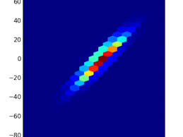
http://planets.utsc.utoronto.ca/~pawel/pyth/fit-3par.py solves the linear least-squares fit problem. The function has 3 parameters (amplitudes) multiplying a parabola. Data have a moderate amount of noise added. Program restores the parabola, hence denoising the data.


http://planets.utsc.utoronto.ca/~pawel/pyth/fit-4parN.py solves the linear least-squares fit problem. The function has 4 parameters (amplitudes) multiplying a parabola plus a cosine function of known period. Data includes noise. Program successfully restores the hidden truth (line), hence denoising the data.
http://planets.utsc.utoronto.ca/~pawel/pyth/fit-4par-N2.py solves the linear least-squares fit problem. The function has 4 parameters (amplitudes) multiplying a parabola plus a cosine function of known period. Data has a large amount of noise added, making it visually difficult to separate smooth functional dependence from quasi-Gaussian noise. Despite this, program fairly successfully restores the smooth underlying function/denoises the data, although the quality of parameter restoration starts to suffer (esp. curvature a[0] is too low).
http://planets.utsc.utoronto.ca/~pawel/pyth/fit-glx-4+2b.py solves the linear least-squares fit problem of dark matter in a synthetic galaxy. The subject is discussed in
http://www.astro.caltech.edu/~george/ay20/eaa-darkmatter-obs.pdf
https://en.wikipedia.org/wiki/Dark_matter
Read the descriptions inside the code. It has several functions for computing
4 separate contributions to the V(R) - the rotation curve of a galaxy, for
a summed up rotation curve, and for plotting the map of errors in the plane
of two parameters which are characteristic scales of the disk and dark matter halo. The 4 components are: supermassive black hole in the center, stellar bulge,
stellar and gaseous disk, and the dark matter halo. The total number of
parameters found by the program is 6.
Plots produced by this 220-line code (with comments of course) show the obtained
values of characteristic masses of components, and the two length scales.
1.
http://planets.utsc.utoronto.ca/~pawel/pyth/err_diff2-sqrt.py
 (click to
enlarge)
(click to
enlarge)
The solution to the analytical (grey and blue-green/emerald curves) and
numerical part of the problem is shown in the figure. A brief look at the code
will show that it is simple, most of it is plotting instructions for
PyPlot (plt).
2.
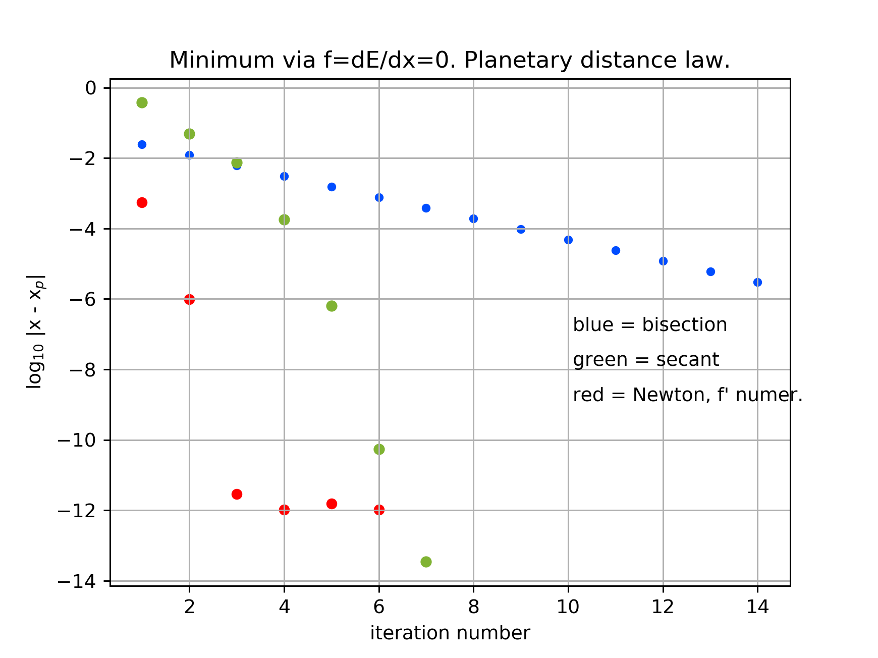
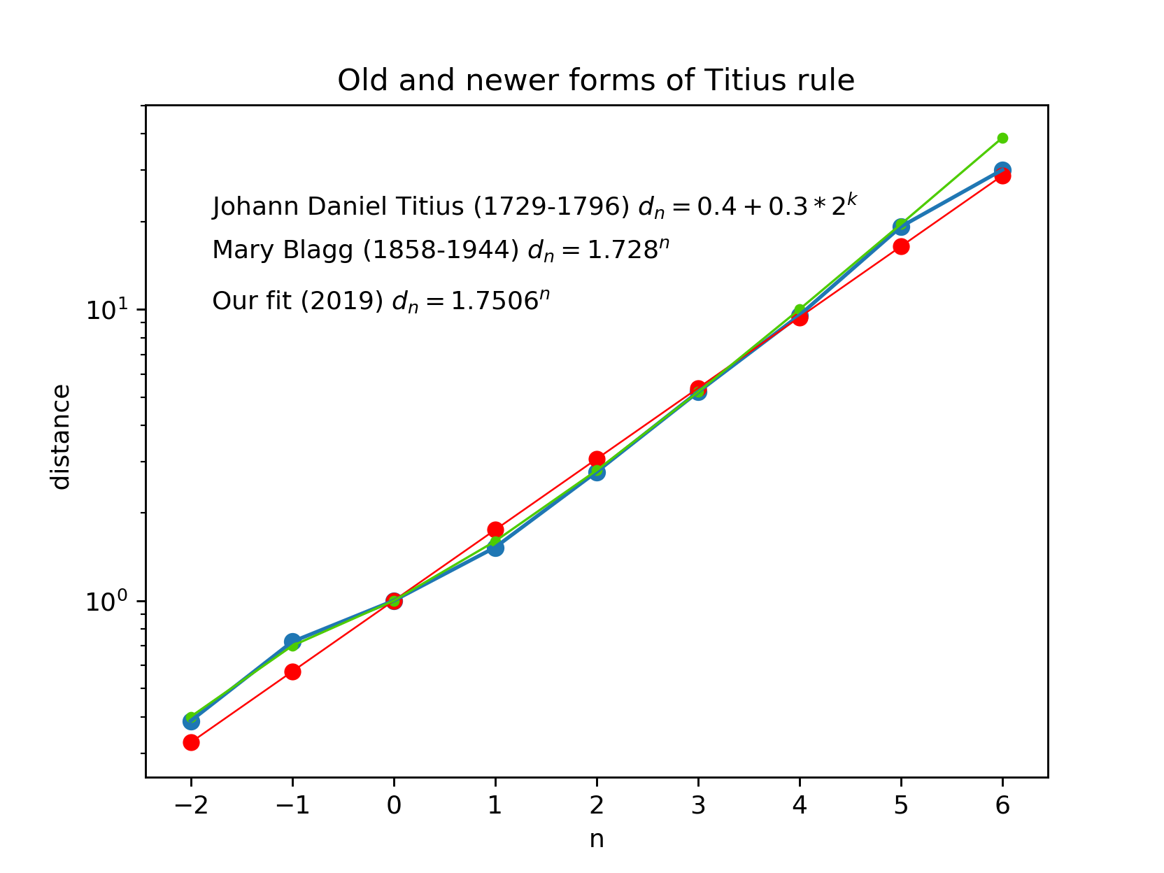
http://planets.utsc.utoronto.ca/~pawel/pyth/Titius-law-3.py
Titius-Bode law.
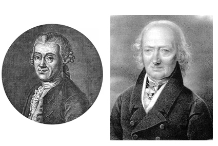
The gentelman on the right (J Bode) published Titius's rule in his popular
book on astronomy. He did not invent it, but in those times
plagiarism or not giving credit was not unheard of, and wasn't considered a
crime. The above code does a little more than the problem asked for:
it presents the convergence study using several zero-finding schemes
(Newton-Raphson's gradient method is extremely quick,
probably because of a lucky first guess),
 (enlarge)
 (enlarge)
and then displays the results of two different formulations of Titius rule,
including the x=1.751 one. Mary Blagg proposed a similar solution
sometimes in 19. or early 20. century.
You can see in the figure when Johann Daniel Titius and Mary Blagg lived.


http://planets.utsc.utoronto.ca/~pawel/pyth/diff1-throw-6.py
This program fort simulates a throw of ball (or arbitrary test mass) in vacuum.
Notice that the air drag will be studied in Lecture 11. Initial conditions:
(x0,z0) = (0,0) & (vx0,vz0) = (70,20) m/s.
http://planets.utsc.utoronto.ca/~pawel/pyth/diff1-ex3.py
1-D ODE integration; solve dy/dx = f(x,y) = -sin(x)*y,
with boundary cond. y(0)=1, & various integration schemes.
http://planets.utsc.utoronto.ca/~pawel/pyth/diff1-ex3L.py
Same as above but
over a 10 times longer period of time. Despite an initially high precision of
some methods, a drift in solution becomes evident. This is bad news, as it is
enough to just wait until the drift destroys the initial accuracy.
http://planets.utsc.utoronto.ca/~pawel/pyth/diff1-ex4L.py
Different equation solved: dy/dx = f(x,y) = -y [sin(x)]^3

http://planets.utsc.utoronto.ca/~pawel/pyth/phys-pendulum.py
Motion of a physical pendulum (able to go to the top and over the top on a
rigid massles arm, depending on initial conditions.
The script implements a Leapfrog algorithm, but looks deceptively simple like
Euler method. Not only does it not do the half-step with positions, full step
velocities and again half-step with positions, but also does not
http://planets.utsc.utoronto.ca/~pawel/pyth/diff1-throw-6.py
The script implements a 2nd order method to perform dynamical simulation of
spherical ball thrown at an angle into vacuum and air
(two different densities of a 5cm-radius ball are assumed: 1200 or 400 kg/m**3).
Drag acceleration = -Cd v|v|/2 rho A/M, an vector proportional to the square
of speed v, directed against the direction of v.
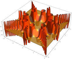
http://planets.utsc.utoronto.ca/~pawel/pyth/lorenz-attractor.py
2nd order method applied to the classical simulation of a chaotic system
of 3 coupled, nonlinear differential equations of order 1. Originally
created to mimic the behavior of quantities encountered in meterological
simulations (convective role), but since then everybody uses it to
illustrate chaotic evolution in general. Fittingly, since this is related to the
Butterfly effect (butterfly flapping wings in Brazil can cause at some future
time a typhoon in Asia), the 3-D plot of the trajectories resembles a butterly.
Notice that this system has 3 variables, really this a minimum number allowing
chaos to emerge. [You must not use this code in the Lorentz attractor assignment
is set #3. Please read the notice in the text of that problem.]
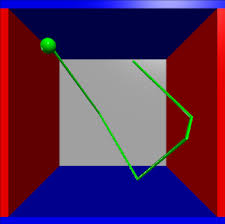
http://planets.utsc.utoronto.ca/~pawel/pyth/chaotic_ball-2.py
The script implements a 2nd order scheme to integrate frictionless
equation of Newtonian dynamics of a common object:
a small mass attached to a point in space by Hooke's spring
(force linearly proportional to extension/compression beyond an
equilibrium length equal of 1.) In addition, unit strenth gravity acceleration
pulls the object down. The trajectory after many up-and-down oscilaltions becomes
extremely sensitive to the initial conditions. You can see how this chaos arises
by changing initial conditions in the eighth decimal digit - you will witness
different first digits in the posion after 100 units of simulated time.
The phenomenon arises because two initially nearby trajectories have tendency
to diverse with time exponentially, thus varying consecutive decimal digits
after a roughly constant time related to the so-called Lyapunov time (corresp.
to the e-folding divergence). As a result, chaotic evolution is
always (by definition) non-periodic.


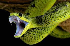
Extension to this problem 1 of the assignment set #4 below. This is the
diffraction-interference pattern from two slits on a screen 1 m away.
Slits are 30 microns wide, spaces 240 microns apart.
http://planets.utsc.utoronto.ca/~pawel/pyth/inteference-1.py
Compare the pattern with the pattern of diffraction on one slit! And click on
the middle illustration above. You'll see the red laser interference fringes
in the actual experiment on the right hand side.
http://planets.utsc.utoronto.ca/~pawel/pyth/pond1.py
This code is deliberately a little buggy and slow. But that's how one would
very naively approach the solution of the 2-D
linear wave equation:
u_tt = c**2 (u_xx + u_yy)
using Python loops (hence slowness!)
http://planets.utsc.utoronto.ca/~pawel/pyth/pond3.py
shows a wave pattern from an initial disturbance of a pond near the corner.
Algorithm uses only Z arrays (different copies for new, current, and
previous time step of array Z.
http://planets.utsc.utoronto.ca/~pawel/pyth/pond4.py
shows a wave pattern from a localized initial disturbance far from the boundary.
This algorithm is only slightly different, introduces explicitly
V array which is first time derivative of array Z (times dt).
Run at about the same speed(?) as pond3.py.
http://planets.utsc.utoronto.ca/~pawel/pyth/pond4-1obj.py
shows that one can force not only boundary conditions on the walls, but also
in the middle, creating a region impermeable for waves.
http://planets.utsc.utoronto.ca/~pawel/pyth/pond4-2slits3.py
This is the famous double slit experiment simulated on water surface or as
soundwaves (no quantum mechanics here, though QM experiment is strictly
analogous and creates diffraction-interference patterns for the same reason.
http://planets.utsc.utoronto.ca/~pawel/pyth/pond4-2slits4.py
Again, Young's double slit experiment.
1.
http://planets.utsc.utoronto.ca/~pawel/pyth/diffraction-1.py
This code solves the diffraction from a single 30 micron slit
2. Aeronautical problem. Fit the drag measurements of an airliner with
two forces: parasitic drag ~ V**2, and lift-induced drag ~ 1/V**2. Derive
certain best speeds from the fit.
Program
http://planets.utsc.utoronto.ca/~pawel/pyth/fit-drag-1.py
solves this problem and displays, first the observational data with
underlying hidden smooth dependencies, and then numerical fit and
optimum speeds derived from the fit. They correspond to the best glide ratio
airspeed, minimum sink rate airspeed, and the Carson optimum speed w.r.t both
time and fuel. See the headers and comments in the program, and L12 notes file.