Tutorials

Tutorials

Tutorial 1

We discussed several examples of non-unique evolution of a 1-d system, by posing and solving two particular dome slide problems.
Please check the 2nd item titled Physics is indeterministic.

Tutorial 2

In the lecture, after comments on the sometimes not-so-great advantage of the potential method in analysis of the 1-D dynamical systems (graphical or analytical analysis of the original equation is usually simpler, though potentials may be very illustrative, esp. about symmetries), we went on to look at

the evolution equation $\dot{x} = rx +x^3 - x^5$ that exhibits hysteresis effect when parameter $r$ is varied.

In the tutorial, we fully solved the physical problem of rotating stand with a horizontally moving bead of mass $m$ under the three forces: centrifugal ($+m \omega^2 x$), large friction ($-\beta m \dot{x}$ much larger in absolute sense than $m \ddot{x}$), elastic force of a linear spring of strength $k$ & neutral (unstressed) length $h/2$, attached on the axis at a level $h$ below the horizontal wire. The frame rotates around the vertical axis with angular speed (or circular frequency) $\omega$. Enlarge and see the pictures:

We introduced a nondimesional coordinate $y = x/h$. There is one parameter controlling the behavior of the bead, a nondimensional rotation rate $\gamma = \omega^2 (m/k)$. Time has been rescaled somehow (it's not important for bifurcation diagram how) and the new time variable is called $\tau$. The method of solution is graphically shown as plotting first $\gamma(y^*)$, and flipping the graph to obtain bifurcation diagram $y_*(\gamma)$.

We got a somewhat strange-looking, but sensible, supercritical pitchfork bifurcation. We did not have the time to add the analysis of the small imperfection of the system, which gives the bead a very small and constant acceleration along $x$-axis. Think of it yourself! I'll ask you about your conclusions. Rotating 1-D systems have been the subject of midterm problems in this course.

Tutorial 3

Total traffic jam at a half-stable fixed point

We solved the following system $\dot{x}=x^2$ to find the time of approach/departure from half-stable point $x^*=0$.

It takes a finite time $t=1/x_0$ to go to $+\infty$ from any positive starting point $x_0$. But when $x_0$ is negative, then it takes an infinite amount of time to very slowly, like $r(t)\sim -1/t$, approach the half-stable point $x^* = 0$ from the left.

Ghost of the half-stable point when $\omega \approx a$

A ghost of this half-stable point is present in the critical slowdown region of the equation $\dot{x} = \omega - a \sin \theta$.

This system actually has an explicit $\theta(t)$ solution that we developed, using Gradshteyn and Ryzhik "Table of integrals, products and series", 2007 edition, 1996 ed.
We computed the period of circulation $T$, it has a very typical dependence on parameters.

Eigenproblems

We considered the eigenvalue problem associated with a 2-d dynamical system represented by 2x2 matrix of coefficients A $$\dot{ {\bf x}} = A {\bf x}$$

The first matrix considered was representing system (if I remember correctly)
$\dot{x} = x + 2y$
$\dot{y} = 4x -2y$
..but no snapshot of the solution seems to have survived :-(. Fixed point (which for such equations is at the origin of coordinates, but in general could be somewhere else if constant terms were added to the r.h.sides) was the saddle point. One eigendirection was along the vector $(0.9,1)$ or so, corresponding to eigenvalue $\lambda_1\approx +2.3$ (the direction is a linear trajectory of exponential departure from the fixed point). Another eigendirection $(-0.5,1)$ or so, corresponding to eigenvalue $\lambda_2\approx -3.5$ described a straight-line trajectory of exponential approach to the same saddle point. The point is unstable in Liapunov sense (see textbook) so to us it is unstable. Remember that eigendirection can be obtained by either by assuming $y=1$ or $x=1$, they are lines, so arbitrarily rescaling ${\bf v}_{1,2}$ vectors is allowed, only the slope $y/x$ matters, and that won't be affected of whether we choose $x$ or $y$ to be 1.

The second matrix considered was representing system
$\dot{x} = y$
$\dot{y} = -2x$

This system has $\tau = \lambda_1 + \lambda_2 = 0 $, and thus two oppositely signed, imaginary eigenvalues $\lambda$. The fixed point is a center, and purely real solutions are following from any real-valued initial $(x,y)$ coordinates.
Do not be worried in such cases that eigenvectors have imaginary (in general, complex) values! Carry on the math. It's ok, they do not represent any straint lines in the phase plane. Trajectories are ellipses or spirals, in general.

Tutorial 4

We looked at one or two nonlinear phase portraits.

Then we followed the Theory of Flight [Dynamics] on our Etudes quasiblog, topic 3.

Tutorial 5 was a midterm

Solutions have been posted.

Tutorial 6

Part of tutorial actually took part during lectures.

Gradient systems as curl-free flow systems

Today during the lecture we solved 7.2.5 from the textbook. The proof one way is trivial, by substitution you prove that if the system is a gradient system, i.e. $f = -\partial V/\partial x, g= -\partial V/\partial y$, then $\partial f/\partial y = \partial g/\partial x$, because derivatives over $x$ and $y$ commute, that is the order of operators in a second derivative does not matter.

The other way the proof is more difficult. I forgot how the companion book proves that $\partial f/\partial y = \partial g/\partial x$ is a sufficient condition for $(f,g)$ being a gradient of some function, but I suspect that the proof below is more sound mathematically and actually tells you how the potential $V(x,y)$ can be computed.

We use the Stokes theorem that states the equivalence of area integral of curl $\vec{f}$ with the line integral of the vector field $\vec{f}$ (in our case that would be $\bf \dot{x}$) over a closed curve forming the border of a 2-d area $A$. $$\int \int (\nabla \times \vec{f}) \cdot d^2\vec{A} = \oint \vec{f} \cdot \vec{dl}$$ Here, $\vec{dl}=(dx,dy)$ is the line element of the closed curve, while $d^2\vec{A}$ is the oriented area element (normal vector of length $dx\,dy$).

In a dynamical system where ${\bf \dot{x} = \vec{f} } = \{f,g\}$, and $\partial f/\partial y = \partial g/\partial x$, the rotation of the vector field has only one component (perpendicular to the $x,y$ plane) and value $|\nabla \times \vec{f}| = \partial f/\partial y - \partial g/\partial x = 0$, therefore the area integral equals zero, and it follows that the circulation (line integral) is also zero, for any closed curve over which we integrate. The only case where that is not true is when the closed curve goes around a fixed point that is a circle, so we have to insist that the the domain that we discuss does not have them. (The more times we go around the circle fixed point in the same direction, clockwise or otherwise, the more line integral value we accumulate, and the integral is not unique.)

From that it follows (I think I didn't say that during the lecture!) that the line integral from one point in the pahse plane to another is a unique functional of those two points. Let's take as the first point, without restricting the generality of the proof, the origin $(x,y)=(0,0)$. Then the line integral from (0,0) to any point ${\bf x}=(x,y)$ does NOT depend on the path taken. Let's prove it.

Imagine two different path, and form a closed loop of them (go to the point ${\bf x}$ one way, and return to the origin on any other path). The result of the integration over the loop is zero, under our condition that curl (rot) of the flow field vanishes. Swapping the limits in the second integral, which is equivalent to the reversal of the direction of travel, you see that the difference of two integrals starting from (0,0) and ending at ${\bf x}$ via different (arbitrary) paths vanishes, q.e.d.

That line integral is our $-V({\bf x})$, a unique function of ${\bf x}$: $$ V({\bf x}) = -\int_{\bf 0}^{\bf x} \vec{f} \cdot \vec{dl} = -\int_{\bf 0}^{\bf x} (f \,dx + g\, dy).$$ Nabla operator is just partial differentiation in $x$ and $y$ direction, with which we can go under the integral sign (and use the fundamental theorem of calculus, derivative of integral is the integrated function, $f$ and $g$ in $x$ and $y$ direction): $$-{\nabla} V = -(\partial_x,\partial_y) V({\bf x}) = (f,g) = \vec{f},$$ which proves that under our rotationless (curl-free) flow field assumption, in domains devoid of sources of rotation like center fixed points, our system is indeed a gradient system ${\bf \dot{x} } = \vec{f} = -\nabla V$, and we have even provided a prescription for finding $V$! You may notice that this is exactly the way we compute gravitational or electrostatic potentials of a given force field $\vec{f}$, although in the phase plane that vector is not a "force" but more like velocity of points in phase plane, a typical representation of a 2-d dynamical system. Points move in time in the phase plane, and their direction of motion is everywhere perpendicular to equipotential curves of $V$. In such systems, $V$ decreases and can never increase, therefore closed trajectories are expluded.

Perturbations

First, please see the new chapter on "Perturbations: how to solve equations you don't know how to solve" in the Etudes and Variations . We discussed that today.

Hill problem

In the tutorial hour we reviewed the solutions to assignments A2. See the solutions file link on our course page.
At the end, we started talking about something else, namely, building on the A2 problem number 4, we talked about the Hill's equations, which are Newtonian dynamics equations valid locally around the much smaller mass of a binary system of masses turning around their center of mass on circles. So Hill's equations are a local approximation of the circular, restricted 3-body problem (restricted means that the smaller mass is very much smaller than the big one, like in a star+planet system).

You already know that all the saddle points of potential are unstable, even if the system is uniformly rotating (as it is here - we go into the frame rotating with two massive bodies and consider the motion of a massless test particle in such a system). Three colinear Lagrange equilibrium points L1..L3 are keeping a constant, colinear, configuration with the centers of massive bodies. They stand still in a corotating system of reference. And they are saddle points of effective potential, so - dynamically unstable. In case the motion starts from the vicinity of such L point, there is a preferred direction, given by the eigenvector belonging to the positive, real eigenvalue $\lambda$, in which the test particles leave the close vicinity of L1 or L2 point (L1 and L2 are equvalent in Hill's equations, there is mirror symmetry).

You are asked to find the unique direction in which particles (gas particles, meteoroids, or spacecraft placed at L1,2 points) flow, while leaving the equilibrium points. A secondary issue: what is the timescale on which the distance from the L point increases $e$ times (think of J. Webb telescope placed near L2 point!). By how many degrees is that direction inclined to the x-axis joining the massive bodies?
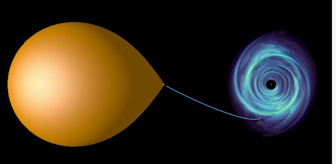
Hint: it's not zero. Astronomer have clever ways of seeing the flow direction and what happens with it after it approaches a masive body (star or planet), which are equivalent to computerized tomography. One difference is that, unlike in a binary system of stars, in a CT scan the detectors (line of sight) rotate around you, not the other way around.

Tutorial 7 on 3 March

We solved the Hills eigenvector problem posed above (direction of streaming from near-rest around L1, L2 points), but got into trouble with arithmetic. Partly my fault, since I suggested to use symbols that did not clearly distinguish time-variable coordinates x,y, from the constant eigenvector components. This is all straightened out in the new topic of the now, take a look at Etudes and Variations, the "Roche lobe overflow as eigen-problem at L1 saddle point" topic.

Tutorial 8 on 10 March

Dog and duck - Etudes

We won't discuss it here, but it's an interesting example of the usefulness of complex numbers (including calculcus in such numbers). For instance, with real numbers, in order to transfer from the inertial frame to the rotating frame attached to the duck, you need to apply a 2x2 rotation matrix to all coordinates. In complex plane, old position vector $z=x+iy$ just gets multiplied by $e^{-i \Omega t}$, where $\Omega$ is frame rotation (angular) speed.

Chaos in Hills equations - Etudes

We discussed that, and I have shown examples of families of trajectories that arise inside and outside the Roche lobe of a planet, where the particles are starting far from the planet on a circular orbit around star (in Hills equations its a vertical trajectory).

Numerical methods - leapfrog method

Use the simple yet robust leaprog scheme whenever you can. It applies to dynamics of particles such as $\ddot{\vec{r}} = \vec{f}(\vec{r}, \vec{\dot{r}})$.

Newton's method: Problem 10.1.12

We discussed that method on thhe blackboard. I don't think we carried out the proof of the superstability (very fast convergence of the method, faster than exponential). I've created yet another Etudes and Variations section, take a look near the end! Link.

Tutorial 9 on 17 March

Quadratic map

We talked of the important difference between Julia set and Mandelbrot set view of any discrete maping. In each case, coloring of pixel representing complex numbers (horiz. axis = real part, veritcal = imaginary part) is quite arbitrary. The point is to illustrate with different colors the asymptotic behavior of the iteration: for instance, using black for diverging series $z_n$, and assigning different colors to period-1, period-2, ..., period-infinity (chaotic) behavior at larege $n$.

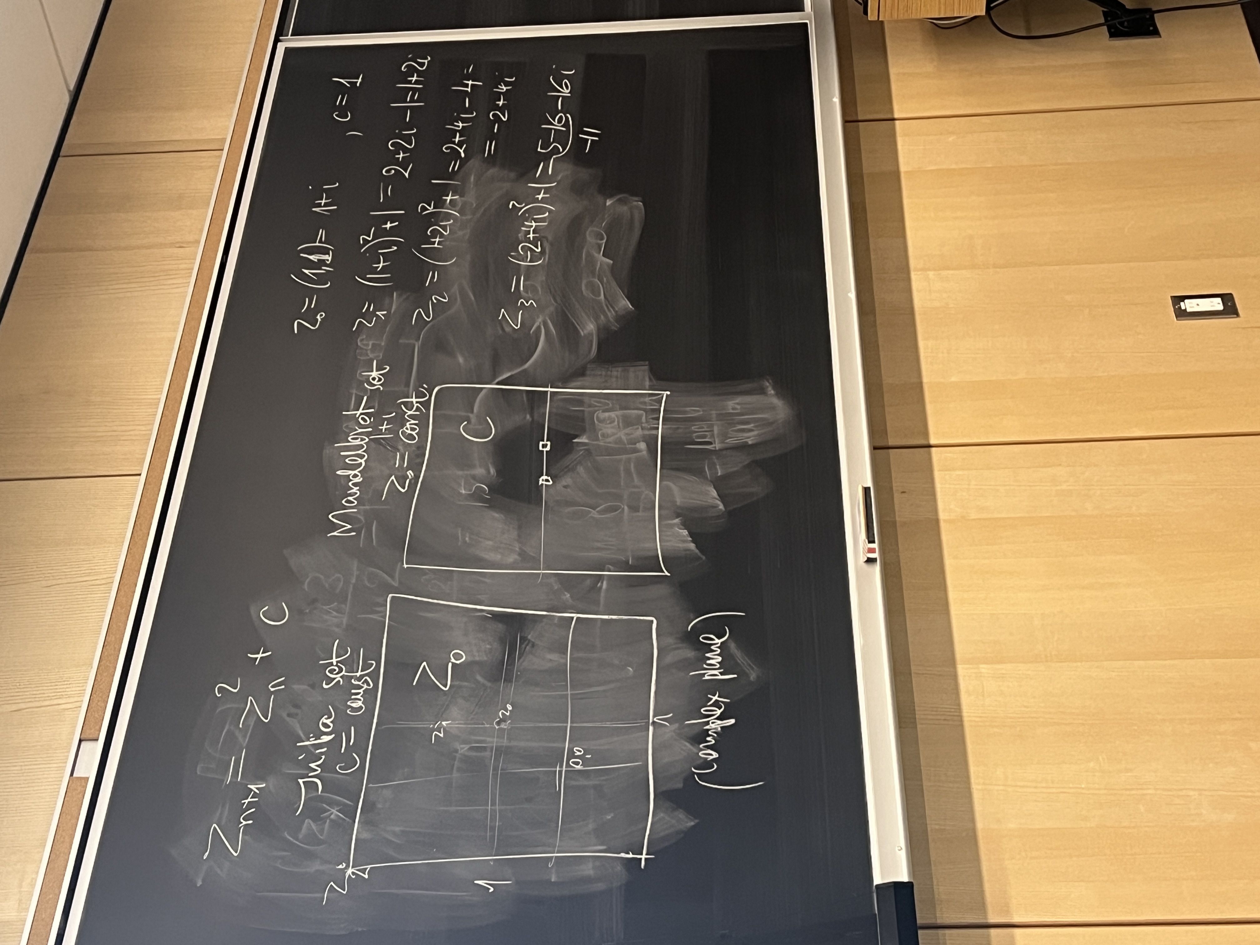
But while the Julia set fixes parameter $c$ and explores all (complex) starting values of the iterated variable $z$, the Mandelbrot set fixes $z_0$ (usually at zero value), and explores in the plot all possible values of $c$.

Sine map

Discrete map $z_{n+1}= 1+(1/2)\sin z_n$ is analysed below. Only one fixed point exists, of unknown stability. Equation for $z_*$ cannot be solved analytically. (Incidentally, and totally unimportantly for this exercise, this is the Kepler's equation for eccentric anomaly studied in orbital mechanics of an elliptic orbit with eccdentricity 1/2, at the mean anomaly = 1 rad.) One can get an $O(y^4)$-accurate approximation to $z_*$ analytically; $y$ is the small (as the figure below convinces us!) deviation of $z_*$ from $z=\pi/2$. We did not evaluate $y$ but have satisfied us that it can easily be found by solving a quadratic equation. Taylor expansion of $\cos y$ skipped terms of order $O(y^4)$.

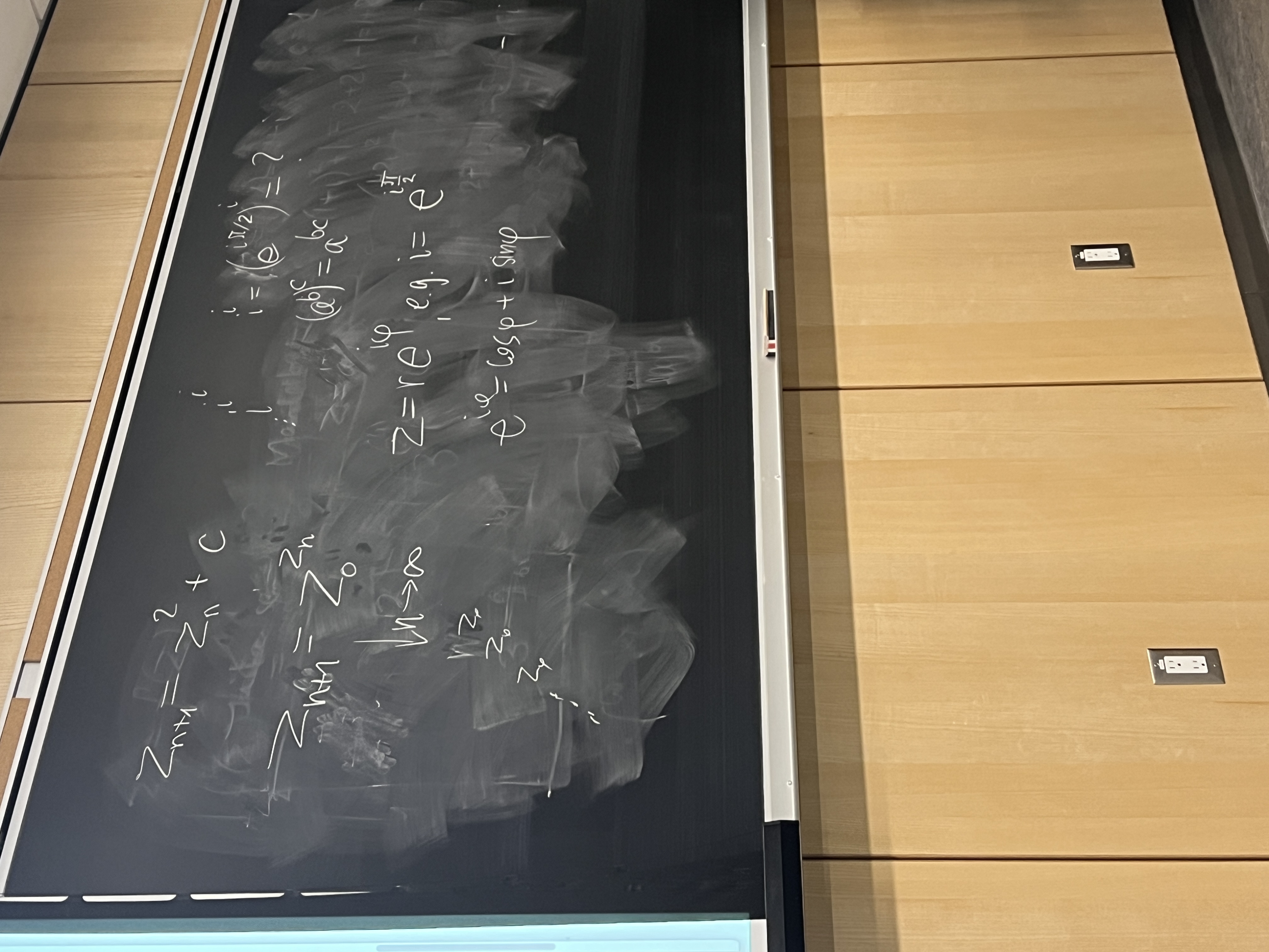
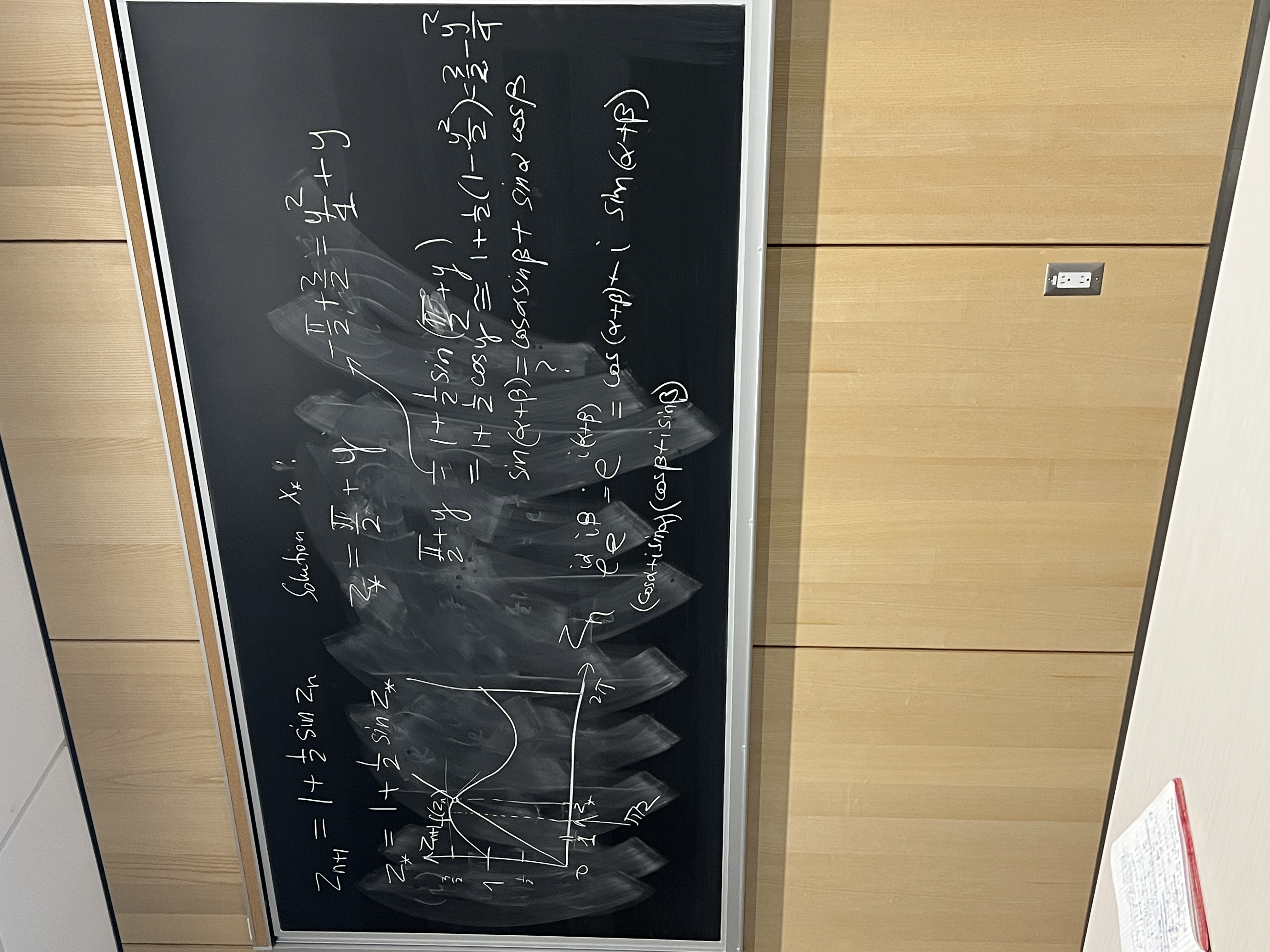
Here is the proof (again!) that $|f'_*|\lt 1$ is the criterion for stable fixed point of any nonlinear mapping, if that first derivative is non-zero of course (otherwise, higher derivatives need to be included and stability type established):

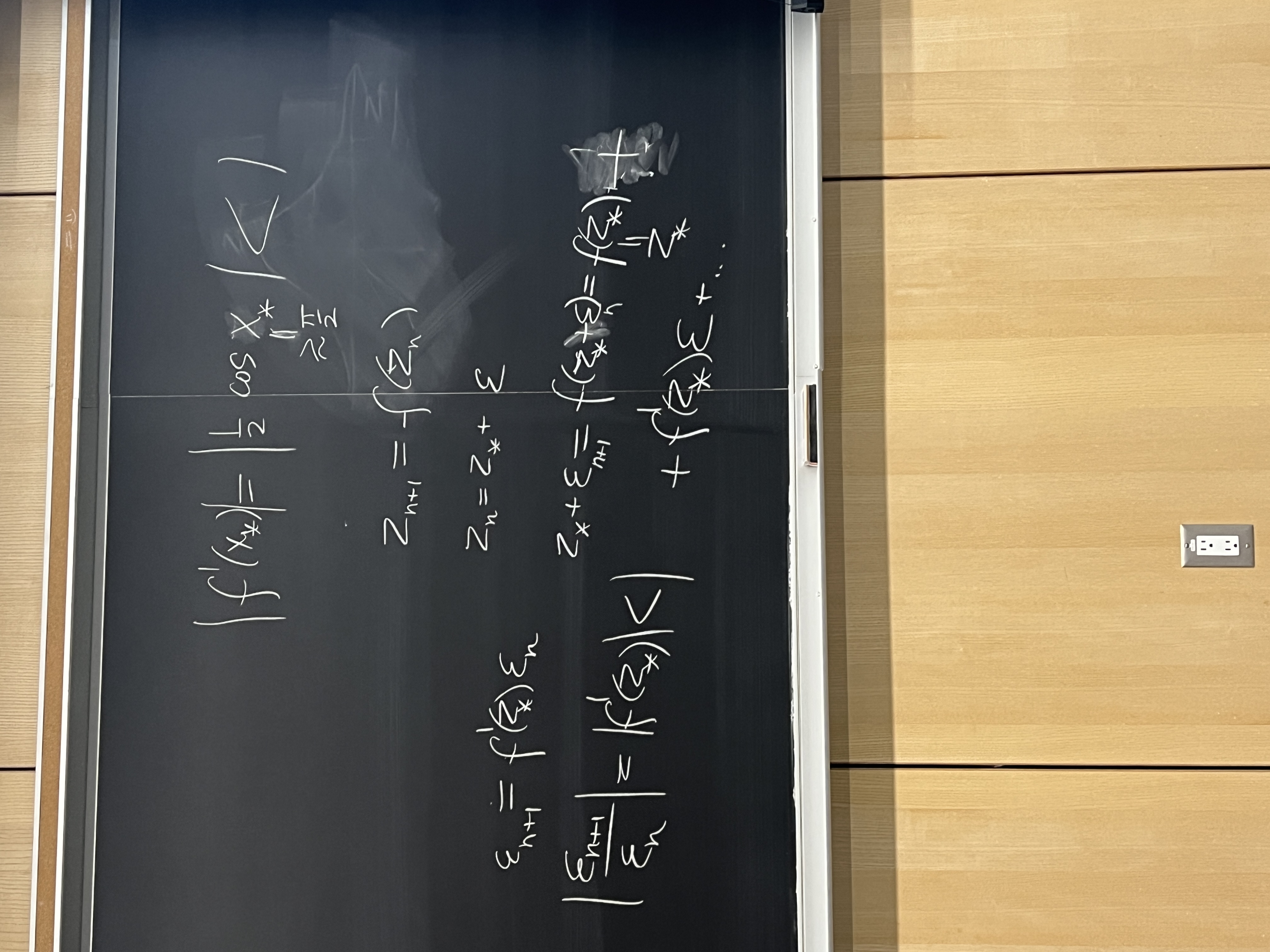
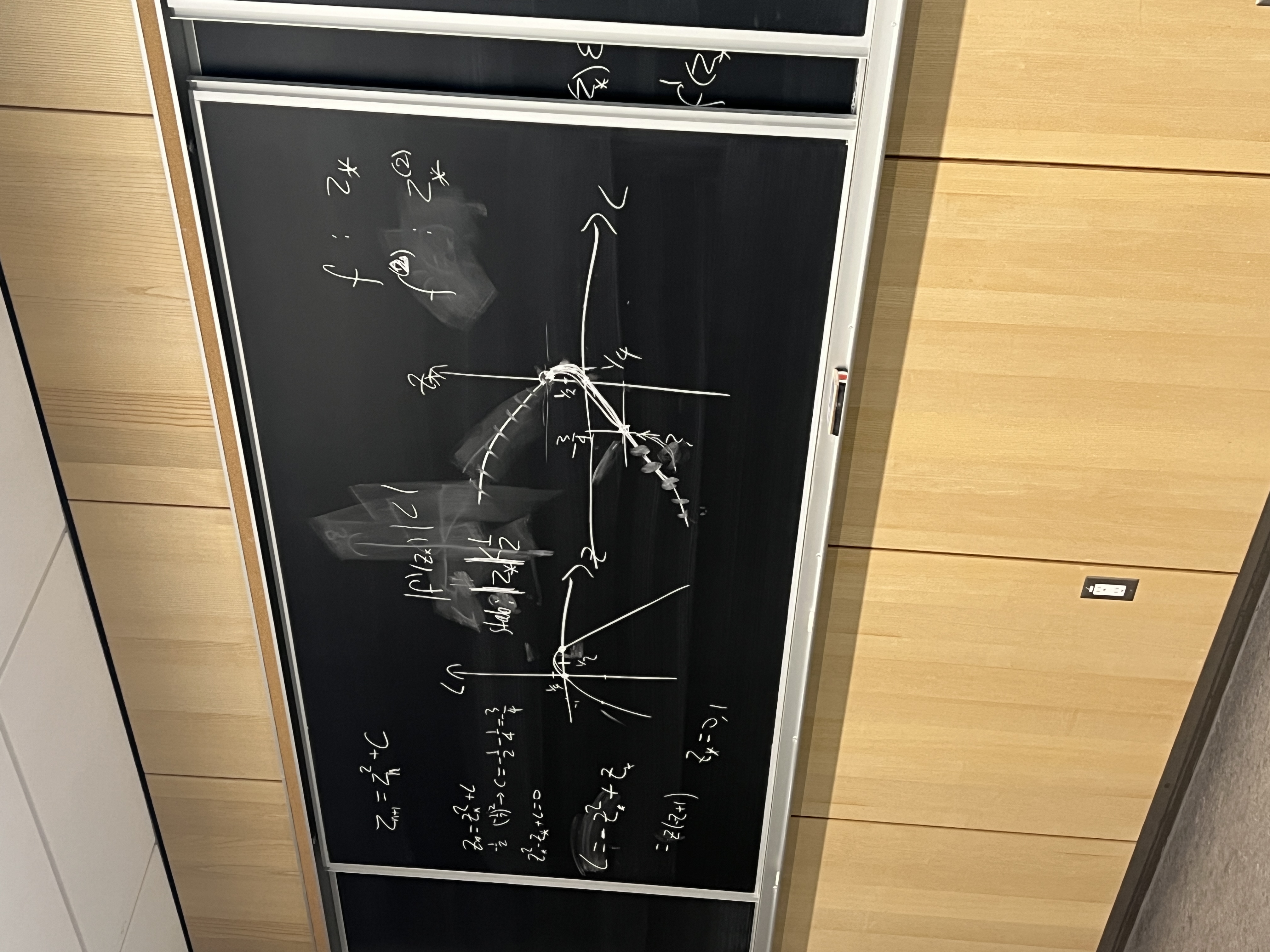
This criterion is applied to the quadratic mapping (relevant to Julia and Mandelbrot sets)

We also talked about the $..i^{i^{i^i}}$ infinite exponentiation series. We even wrote a Python script to display its progress in complex plane. Take a look at the Etudes and Variations blog, the last chapter titled "How to compute a new math constant fast".

The exponential fractal

In lecture & tutorial we discussesed fractals, and watched this video illustrating many well known examples.

See the description of 'my' self-exponentiating fractal . We reviewed this, but fankly someone should do an animation of a zoom into it. It was technically impossible to do thousands of frames for such a video in the 1990s. The self-exponentiation fractal is arguably more beautiful than the Mandelbrot one.