In order to achieve higher accuracy and better speed of execution, evaluate the
r.h.s. twice and average the f's at the beginning and end of subinterval dt.
f0 = f(x,t)
; high accuracy f at the starting-point
xend = x + dt * f0
; low accuracy (1st order) prediction of endpoint x
f1 = f(xend,t+dt) ; quite high
accuracy endpoint value of f
x = x + dt*(f0 + f1)/2 ; high-accuracy
(2nd order) prediction of endpoint x
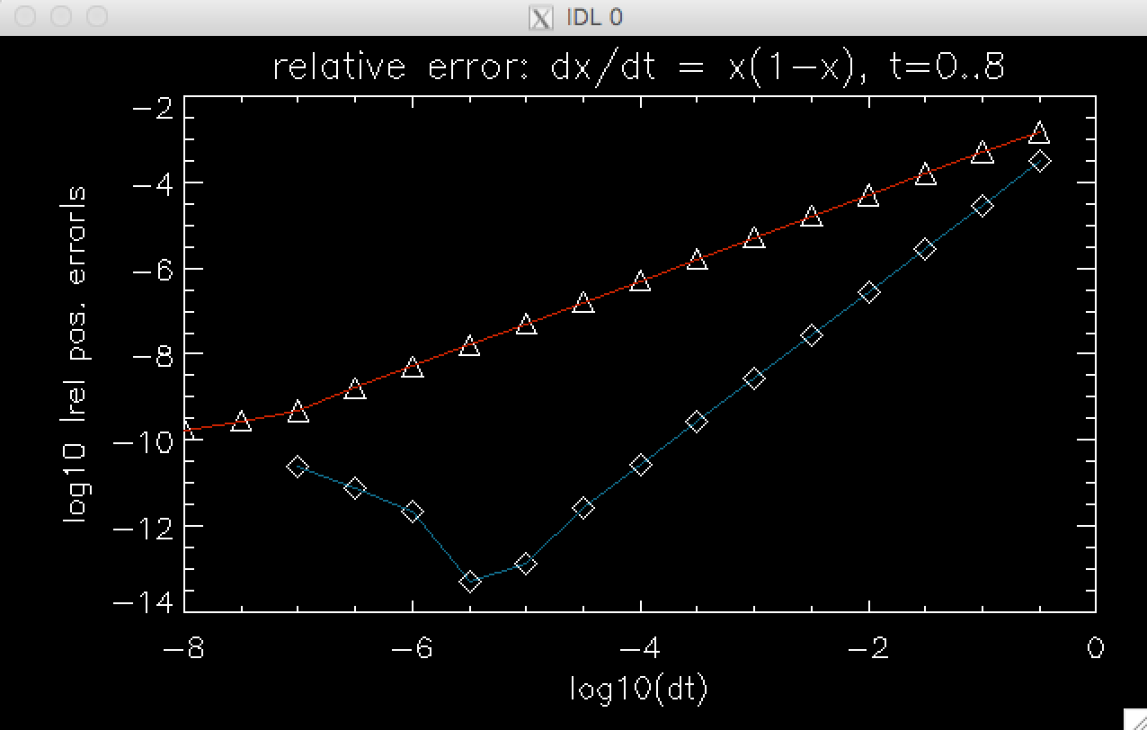
The above is a 2nd order accurate integrator, one of many. That means the error is of order O(dt2), i.e. faster convergence with diminishing dt than 1st order scheme can provide. It's called the trapezoid method.
There is also a midpoint scheme, where first r.h.s. evaluation is used to get an accurate x-midpoint at time t+dt/2, and then r.h.s. is re-evaluated to get an accurate estimate of f(xmid,t+dt/2), i.e. the average f over time from t to t+dt (this f is used for the final update of x). Midpoint scheme is also of 2nd order accuracy.
The diagram shows the accuracy as a function of dt (on log-log plot) for the trapezoid and the 1st order Euler scheme. Click to enlarge. Make sure you understand the slopes of the two curves, representing what we call a truncation error (in the sense of truncation of Taylor series. It's simply an error caused by limited accuracy numerical scheme and the necessary discretization of time.)
The reason the blue scaling breaks down and the red one levels off at very small dt's is the roundoff error in computer double-precision arithmetic. The more timesteps you take, the further you random-walk away from the true solution.
Finally, try this crazy idea and see if you can save some computational time by
doing only 1 evaluation of r.h.s. per subinterval of time (dt) -- the
evaluation is usually the most expensive part of the algorithm -- and still get
2nd order accuracy!
xmid = x + (dt/2)*f ; use f from previous time step,
low accuracy
f = f(xmid,t+dt/2) ; quite high accuracy midpoint f
x = x + dt * f ; high-accuracy prediction
No, you won't succeed... :-( This is still a 1st order scheme. If you could remember more old values of force (a multistep scheme), you could make a better prediction of midpoint x by effectively estimating the rate of change of the r.h.s., and have a higher order scheme while doing only 1 new evaluation of the r.h.s. per dt.
Amazingly, something like this unsuccessful trick does work for 2nd order ODEs like Newton's momentum equation dv/dt = f(x,t).
The simplest 1st order integration scheme is to turn one 2nd order ODE into two
1st order ODEs.
v = v + dt*f(x,t)
x = x + dt*v
In this form, if we take care to start (and later end) the computation in [0,T]
time interval with de-sychronizing operation v = v + (dt/2)*f(x,t) ONLY in the
first step & very last timestep (with no x-update), then our v's will be
evaluated at midpoints of the time intervals [t,t+dt], while x's at the ends
only. Positions and velocities will be leapfroging over each other,
as we proceed through time. The scheme is called leapfrog integrator and is 2nd
order accurate. It is symplectic (preserves energy very accurately with no
systematic drift).
If however you swap the order of the v and x updates in the above scheme, the accuracy is only 1st order. So, just in case, remember to always update velocities first. Even if you forget to desynchronize variables at the beginning, along the way your scheme will have 2nd order accuracy.
But in tutorial 1, we saw examples of indeterminism of physics even in its simplest form: classical Newtonian mechanics. One can certainly give many other examples, but lately the problem of object rolling or sliding down form the top of an axisymmetric dome has been used for illustration & discussion, for instance in this science video-blog.
Here are the calculations of what happens to an object sliding on a dome of the
shape given by function $h(r)$ in two cases. The first is
$h=-r^2/a$, where $a = const.$ scale length.
 .
.
In this case the mass has zero total kinetic+potential energy (to be able to
sit at the top of the dome at rest). Two types of solutions are possible but i
there is no mixing of them, at least not in a finite time. They cannot be
spliced to form one compound history including two types of behavior (A and B),
forming a continuous function of time, satisfying the Newtonian dynamics laws.
The second is a dome with the fractional power shape:
$h=-\frac{2}{3}
\beta^{-1/2} r^{3/2}$ ($\beta = const.$ scale length)

This case is very different, in that a quartic function $(t-t_0)^4$, the part
which describes an ascent to the top, can be connected to an arbitrarily long
stretch of second type of solution, and then back to the quartic solution
describig a descent. In addition to this considerable arbitrariness, the
azimuthal directions of ascent and descent can differ by an arbitrary amount.
In the past centuries, classical mechanics was considered deterministic. That is, given a set of initial conditions, and the differential equations of dynamics, the future of the physical system was supposed to be fully knowable. (Remember Laplace's deamon?) But it isn't. The non-uniqueness of solutions that start from fixed initial conditions is seen in the second dome problem (and many other). It is the sign of indeterminism in Newtonian physics.
So what are the conclusions from this exercise? Does it mean that the world we live in is indeterministic and the future unknowable? Well, our exercise does not prove that. Physics and the world are not precisely the same thing. Physics with all its simplifications and implicit assumptions is just a language in which we talk and think of a very complicated universe. But it's very suggestive, isn't it?
Notice that our $D/L$ stands for the ratio of coefficients of drag and lift, but more generally it is the ratio of forces (proportionality of both forces to v2 is not required.) A steady-state glide happens at $\theta^* = -D/L \sim -1/30$ rad (-2o) for good gliders, and less than 1.5o for the winning gliders. Polish glider called Diana 2 has a fantastic max glide ratio 50:1, meaning -1/50 rad = -1.15o glide. For comparison, a typical older airliner (like Tupolev TU-154 or Boeing 767) will glide some 17 times further than it sinks, at an angle 3.4o to horizon. For that reason, standard final glide paths to airports tend to have a prescribed slope of at least 3o, typically 3.5o, so that a jetliner with engine malfunction has a chance to retract flaps, fly at optimium speed, and land on a runway faster than usual but in one piece. Flaps are needed for nice and slow landing. They increase drag by a larger factor than lift, which spoils the aircraft's aerodynamics (here, L/D); on a standard approach the jetliner must thus keep a noticeable fraction of engine thrust to maintain the prescribed shallow glideslope. If you live near the approach path to an airport, you may have noticed it.
More modern designs like Boeing 787 Dreamliner advertise glide ratio 21:1 (-2.73o), which happens to be close to the performance of an excellent soaring bird albatross, who has L/D ≈ 22, so θ* ≈ -1/22 rad or -2.6o. Albatross can soar 1000 km a day. Its flights take it around the globe. To reach such high glide ratios L/D, wings must have a very elongated shape. That's why both gliders and albatrosses have such wings. The wingspan of the latter reaches 3.4 m. Also, to keep wings fully extended albatrosses have a special lock on the tendons, and do not use muscles to keep wings steady; they use ascending air currents and winds, and do not waste energy on flapping their wings either, unlike sparrows, who have a horribly bad L/D = 4 and sink 1 m per every 4 meters covered in gliding. OK, from birds, gliding frogs and flying fish, back to our equations, via a brief interlude on piloting and landing an airplane.
Look at the θ* equation: $\theta^* = -D/L$. You want to reduce |θ*|, so you need to reduce the D/L ratio. Lv2=W in stable flight (lift = weight). The only way to reduce $D/L= (Dv^2)/W$ is to add engine thrust force or rather, acceleration T, to reduce $Dv^2$ (acceleration of parasitic drag) by T. In no case should you re-trim the airplane or pull on the controls to raise the nose, while leaving the thrust unchanged. That will only INCREASE the total drag (by raising the so-called induced drag), lower the speed, and reduce your range. Even though the nose will be pointing higher (say, in the direction of the runway), fooling you to believe that you're now doing better, you will actually sink faster and crash short of the runway. Which will spoil your whole day.
Another issue is the speed. Let's say you glide and suddenly notice on the
airspeed indicator that v=v* is dangerously low, too close to the stall speed
of the aircraft, below which the smooth airflow is guaranteed to detach from
most of wing's surface (L drops, D goes up dramatically, and the wing is more
falling than flying). You need to correct v* up to the recommended, safe, value
equal 1.3 times the stall speed.
Car drivers have an intuitive reaction to step on the gas, in order to speed up.
Very wrong, again, in aviation! If you do increase engine power, the thing you
change is $\theta^*$ (which we just covered), but the speed $v^*$ won't go up.
Since $v^* = (g/L)^{1/2}$, what you need to do is to lower the lift
coefficient $L$, which depends on the angle of attack rougly linearly.
You do that by pointing the nose down, which reduces the angle of attack,
the lift coefficient $L$ (and part of drag called induced drag).
Congratulations, you saved the day avoiding a stall-and-spin accident!
There is a lot of nonlinear physics in flying. For an example of aerobatic maneuvers such as rolls, loops and an immelman (half-loop + half-roll) see a video with your prof. instructing a friend in an aerobatic-capable plane RV6A. To find out more, check the basic and advanced aerobatics textbooks.
The trace of matrix A is negative,
τ = tr A = $-3Dv^* < 0$,
whereas the determinant is always positive:
Δ = det A = 2(Lv*)2+2(Dv*)2 > 0.
Considering that if D/L ≪ 1, then τ2-4Δ < 0,
we have established that the glider is in a stable equilibrium
(cf. the classification of linear nodes on p. 138 in the Strogatz textbook).
If you don't believe that, convince yourself step by step, writing down the
eigenproblem fully:
A x = λ x, or (A-λ I)x = 0, where
I is a unit 2x2 matrix.
Non-trivial solutions exist only if det(A - λ I) = 0, which
we write out as the characteristic equation
λ2 - τ λ + Δ = 0
that yields two eigenvalues λ1,2. Writing this quadratic
function of λ as
(λ-λ1) (λ-λ2)=
λ2 - (λ1+λ2) λ +
λ1λ2,
and comparing that from with characteristic equation we see that
the sum of eigenvalues equals τ and is negative, while their product
Δ = det A is positive. But λ1 and
λ2 are not simply two negative real numbers.
Inequality τ2-4Δ < 0 implies that they are a pair of
complex-valued eigenvalues, because the explicit solutions of the quadratic
equation for λ's are
$$ \lambda_{1,2} = \frac{\tau}{2} \pm \frac{i}{2} \sqrt{4\Delta - \tau^2}$$
The expression under square root is positive. The imaginary parts have opposite
signs; we can construct sinusoidal oscillations from them. Most importantly,
the real parts of eigenvalues are equal and negative: τ/2 < 0.
This tells us that both independent solutions are damped in time (how fast,
we will see below). The equilibrium point of the 2-D dynamical system is
classified as stable spiral, and the flight of an airplane or bird is
self-stabilizing.
As will become evident soon, we have found a fairly slow oscillation of an aircraft in flight, involving only pitch changes but no bank, both features distinguishing this mode from a faster, longitudinal+lateral oscillation called Dutch roll. It is known in aerodynamics as phugoid or phugoidal oscillation. We will further analyze phugoid oscillations below, after a historical interlude.
Lanchester's early aerodynamical paper "The soaring of birds and the possibilities of mechanical flight" was written in 1897, much before the first airplane was built. He was ahead of his time. [In 1927 he also designed a hybrid, "petrol-electric" passenger car; trucks used hybrid engines even earlier! One of such trucks pulled the telescopes up a dangerous path to Mt. Wilson observatory from Pasadena, CA, in 1908-1918. But it proved too weak, and was supplemented by an auxilliary donkey in front.] In the second part of a two-volume book on flight published in 1907 and 1908, both on microfilm in U of T library, Lancaster described the phugoid (minus the damping). The phenomenon is described in wikipedia, although in scant physical and mathematical detail.
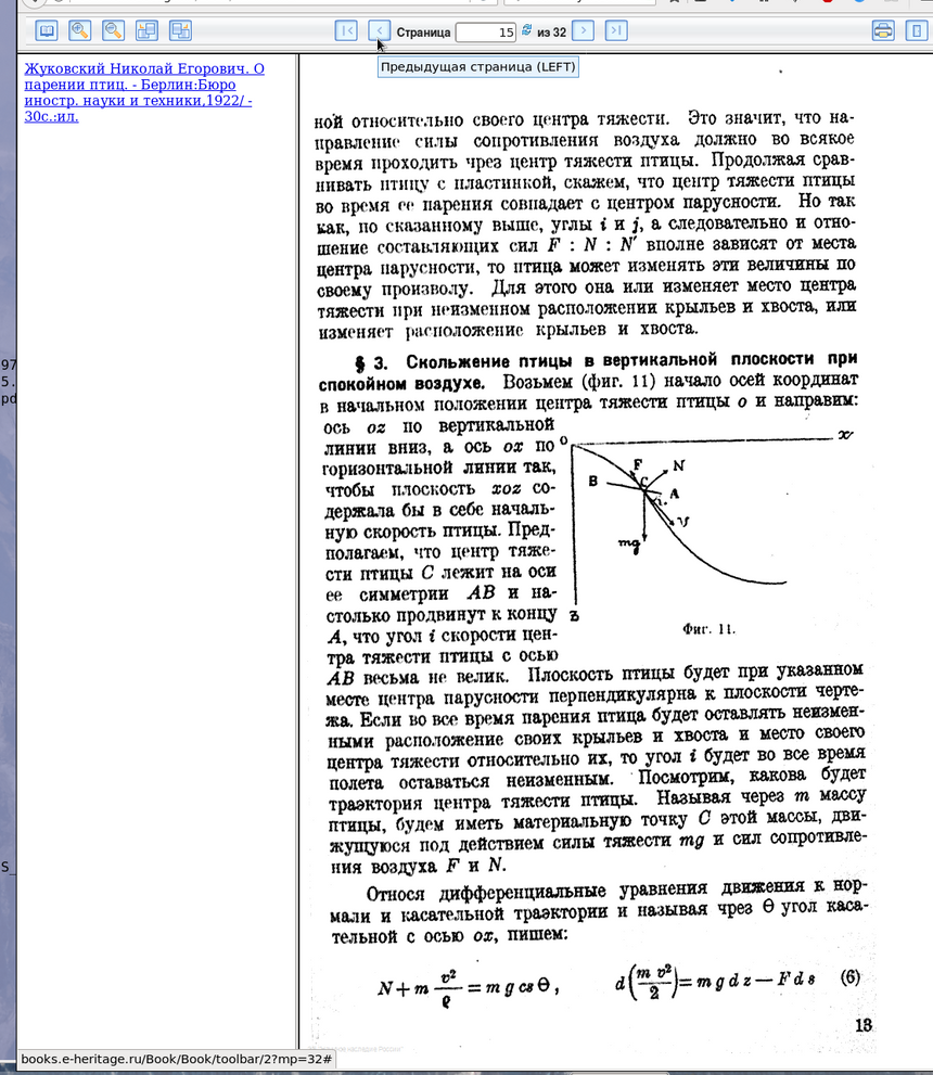
It turns out that a prominent Russian aerodynamicist explained the lift force as a result of circulation of air's velocity field around airfoil. He also studied the theory of phugoid earlier than Lanchester, and predicted the possibility of making loops (before an airplane was constructed), in a paper on gliding of birds. That man was Никола́й Его́рович Жуко́вский or Nikolai Zhukovsky (sometimes spelled Joukowsky).
I have recently dug up Zhukovsky's works earlier and more comprehensive
than Lanchester's (Жуковский Н.Е. О парении птиц. Мoscow, 1891), cf.
this 1922 publication.
It turns out that it was Zhukovsky who first formulated the differential
equations that we set up at the beginning of this story of phugoid oscillation.
He solved them by an approximate method, including the drag force,
which Lanchester ignored (denoted F on the first picture):
 Here is more on
airfoil theorem and the
Joukowsky transform and airfoils.
Here is more on
airfoil theorem and the
Joukowsky transform and airfoils.
By the way, Russian Empire's military pilot Пётр Николаевич Нестеров
(Pyotr
Nikolayevich Nesterov) after convincing himself by calculation that such a
feat is possible to accomplish, performed in 1913 at an airport near Kiev
the first
loop (then called a dead loop) in a French-designed, Russian-built,
70 horse-power Nieuport IV airplane. Initially arrested for unauthorized
use and endangering Army's property, Nesterov was soon released and given on
order of merit.


We already obtained two eigenvalues, which we can evaluate by substitution of
τ and Δ:
$$\lambda =-\frac{3Dv^*}{2} \pm i\sqrt{\frac{2g^2}{v^{*2}}
-\frac{9D^2v^{*2}}{2}}.$$
In the square bracket, the second term is ~(L/D)2 times smaller
than 2(g/v*)2 = 2(Lv*)2 and can be neglected.
We can write the eigenvalue as $\lambda = -t_d^{-1} \pm i \omega$,
where $$\omega = \sqrt{2} \frac{g}{v^*}$$ is the oscillation frequency, and
$$ t_d^{-1} = \frac{3Dv^*}{2} = \frac{3}{2^{3/2}}\,\frac{D}{L}\;\omega $$
is the inverse time of amplitude damping, both constants having the physical
unit 1/s. The time scale td is the e-folding amplitude decrease time
(decrease by factor e≈2.718).
$$P = 2π/ω = \sqrt{2}\, \pi \frac{v^*}{g}$$
is the period of phugoidal oscillations.
Comparing td and P, we get
$$ t_d = 2/(3 D v^*) = (L/D) \sqrt{2} (3\pi)^{-1} P \simeq 0.150 (L/D) P.$$
Phugoid damping in good gliders with L/D > 30 takes
td > 4.5 P, that is more than about 4.5 periods of oscillation.
Badly designed aircraft are actually damping phugoids better, not worse!
In them L/D is lower and damping takes fewer periods. But weak damping of
phugoids is a small price to pay for small drag and high gliding ratio, Besides,
they can be damped by dedicated feedback systems deflecting control surfaces.
Very interestingly, phugoid period P does not depend on anything except the forward speed of flight: neither on how aerodynamic the aircraft's design is (what's its L/D ratio), nor how hot, dense, humid or viscous the air on a given day is, which depends on the atmospheric conditions and flight altitude, etc. The airship does not even have to be a glider, it could in fact be an airplane powered by engine(s). Could you redo the derivation with a constant thrust +f added along the path? This would surely change the equilibrium glide/ascent angle but not the formulae for oscillation and damping periods, in our simple theory. Would thrust change v* much? Do the calculation - you may be surprised and learn a bit about piloting. On approach, pilots most aircraft control glide angle but not the speed with engine thrust. They control speed by changing the AOA of wings with the elevator, a control surface attached to horizontal stabilizer. The stabilizer itself is responsible for short-term longitudinal stability (also damped oscillations), but the time scales of these are an order of magnitude shorter than what we discuss here.
In practical terms, our phugoid formula predicts $$ P \approx \frac{v}{100 {\rm m/s}} \; 45.3 \;{\rm s}.$$
For an airplane flying at 306 km/h = 85 m/s, such as during the approach of flight number PLF 101 of a Polish presidential TU-154M aircraft on 10.04.10 that exhibited large vertical speed and glidepath variations resembling a phugoid (PLF 101 collided with trees and crashed, killing all 96 people on board), we obtain a phugoid period P ≈ 39 s, roughly in agreement with the black box recordings. The phugoid phase was unlucky in that the nose started dropping slightly at a moment when the trajectory should have been corrected in the opposite direction. But it was not a cause of the accident, merely one of contributing circumstances. The crash was a consequence of pilot errors in difficult meteorological conditions in Smolensk, Russia (low cloud base and dense fog). The crew was not supposed to descend below the MDH = minimum descent height, 120 m above the runway, because they had zero visibility there. They continued a too-steep descent until they emerged from the fog and saw the ground just 25 m below them. It was too late to avoid collisions with trees, resulting in loss of a 1/3 span of the left wing, an uncontrolled roll to the left and an inverted crash into a sparse forest. I was analyzing that catastrophe as an independent researcher, supporting the Polish governmental committee. Below is my reconstruction of vertical velocity and altitude deviations in the approach path, which should be smooth and much less steep (or else a go-around must be executed, which wasn't done). The vertical speed and approach cone indicated in green are the mandated ranges in a non-precision approach in TU-154M at Smolensk Severnyi airport (click the images)


Time in seconds is on the horizontal axis in the plot of vz on the
left, and the distance to runway threshold in km is on the horizontal axis
in the figure on the right (altitude above the runway in meters is shown
on the vertical axis).
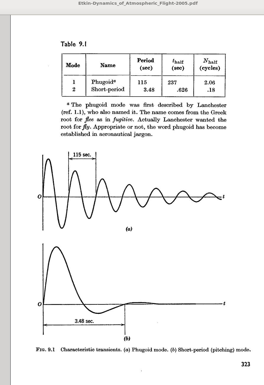
Another example is a flight at cruise speed of 500 mph = 435 kt = 805 km/h =
224 m/s (see Etkin, book "Dynamics of Flight" 2005).
Etkin employs a much fuller set of dynamical equations, actually taking into
account those things we said are not entering our equations, including
all the so-called aerodynamic derivatives and aircraft's moments of inertia of
an airliner. He gets the following answer: phugoid of period 115 s, e-folding
damping over approximately 3 oscillation periods. In addition, the richer
set of equations predicts more eigenvalues and a very quickly damped
short-period oscillation, which we do not predict at all. We get the period
P(500 mph) = 101.4 s. That is a 12% shorter P than from Etkin's calculation.
Incidentally, the 2005 edition is based on a 1972 edition, where the eigenproblem was solved on an computer in those long-gone times when computers were so rare that their use merited a mention in the book; it was an IBM 1130 mainframe computer at UTIAS (that's our UofT Institute for Aerospace Studies. Etkin was UofT Prof. and Dean. He died 10 years ago.)
OK, so we underpredicted the computed phugoidal period (Etkin 2005) shown here,
 and also this
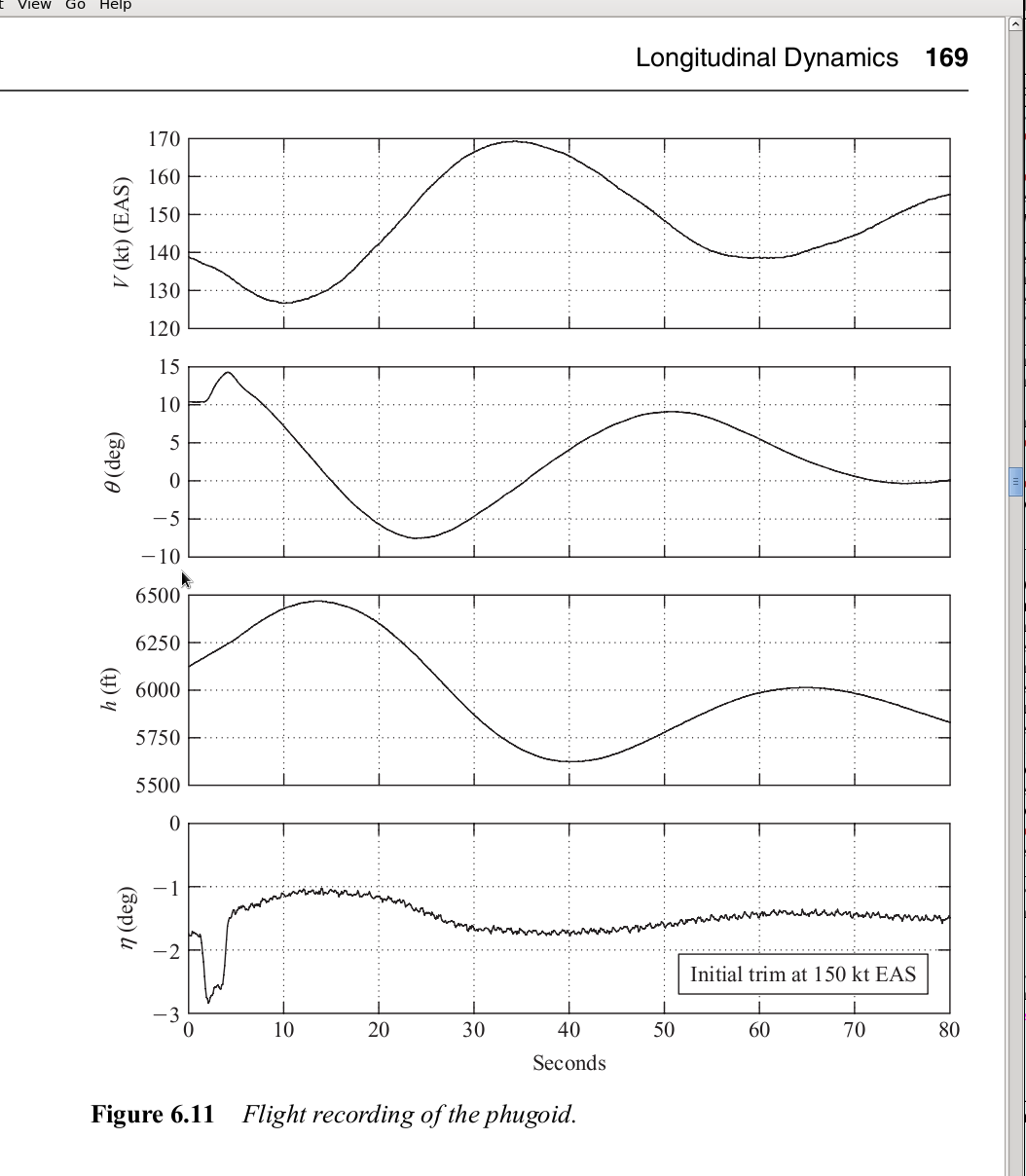 actual flight test measurements at v* = 150 kt, where a small jet was
oscillating in about P = 50 s, while we computed P = 35 s. Nevertheless, our
result is still classical, as it gives the phugoid period exactly the same as
in both the original derivation by Lanchester (1908), who used energy
conservation principle and the assumption that engine thrust exactly cancels
the drag, and in a lot of subsequent derivations making fewer assumptions
than we made, as discussed in aerodynamics books such as Cook's "Flight Dynamics
Principles" (2nd ed. 2007), from which we took the right-hand figure above.
actual flight test measurements at v* = 150 kt, where a small jet was
oscillating in about P = 50 s, while we computed P = 35 s. Nevertheless, our
result is still classical, as it gives the phugoid period exactly the same as
in both the original derivation by Lanchester (1908), who used energy
conservation principle and the assumption that engine thrust exactly cancels
the drag, and in a lot of subsequent derivations making fewer assumptions
than we made, as discussed in aerodynamics books such as Cook's "Flight Dynamics
Principles" (2nd ed. 2007), from which we took the right-hand figure above.
If you want to learn about other types of airplane oscillations and instabilities, they are discussed e.g. here. Phugoids are sometimes shown in videos like this one, but they are so boringly slow that I guess they actually should be shown at 4x fast-forward speed.
Why are phugoids important? Because as already mentioned, unlike the short-period oscillations, the long climb and long descent in a phugoid causes large altitude deviation. A pilot who needs to maintain level flight has one more thing to actively correct, unless the plane is in cruise and is steered by multi-axis autopilot enforcing the longitudinal stability. However, on the final approach autopilots in most airplanes must by disengaged, and in the Smolensk crash it was not controlling the glidepath. Captain Sullenberger, who in January 2009 successfully ditched an Airbus 320 on the Hudson river in NYC, following two bird strikes and a complete loss of engine power, said that the phugoid-control circuit was interfering with his flare (increase of $\theta$ just before ditching the plane). This sounds a bit strange, but who knows. There are no other cases to compare.
SOLUTION
There are different kinds of solutions. One of the previous years, half of students voted for a numerical solution first, and half for analytical solution first. Both are good choices for the first stab, as long as you attempt the other method as well.
As a matter of fact, if you start with numerical solution then you're immediately faced with the problem of what equation to ask the computer to solve. Let's talk about that first, then. I will use a compact kind of notation, using complex numbers in place of vectors, although at the cost of writing twice as many equations one can work directly with (x,y) or with (r,φ) coordinates of the dog in the program. Complex numbers just look.. less complex in a program. You may think of them as vectors, which they are. Let the position of the dog be r = x+iy, and D be another complex number giving duck's position.
The dog goes straight for the duck, so along the vector D-r, at speed s, i.e.
dr/dt = s (D-r)/|D-r|
where the ducks position is known to uniformly move in a unit circle:
D(t) = exp(it).
That's not the end, since both animals are moving in some circular or
quasi-spiral way. Rather than talk about position r(t), we switch to vector R,
R = exp(-it) (D-r)
which is an instantaneous vector from the dog to its moving target, in a
reference frame that rotates at unifom unit speed with the duck. In such a
rotating frame, the duck is always at (0,0) position and R won't run wildly
in quasi-circles, obscuring the plot. The required frame rotation is
accomplished by turning any vector to the right by t radians, which is easily
done in complex plane with multiplication by exp(-it).
We work out, by differentiation of the definition, the derivative of R to be
dR/dt = -i exp(-it) (D-r) + exp(-it) [dD/dt - dr/dt].
Taking into account that dD/dt = i exp(it), and that dr/dt=sR/|R|, we obtain
our evolution equation for a 2d dynamical system in the complex form
dR/dt = s R/|R| + i(1-R)
The numerial solutions for R(t), t=0...500, were obtained with this second-order integrator (dt = 0.004 was sufficient for accuracy), for a series of 20 uniformly spaced values from 0 to 1 (s = 0.05, 0.1, 0.15, ...).
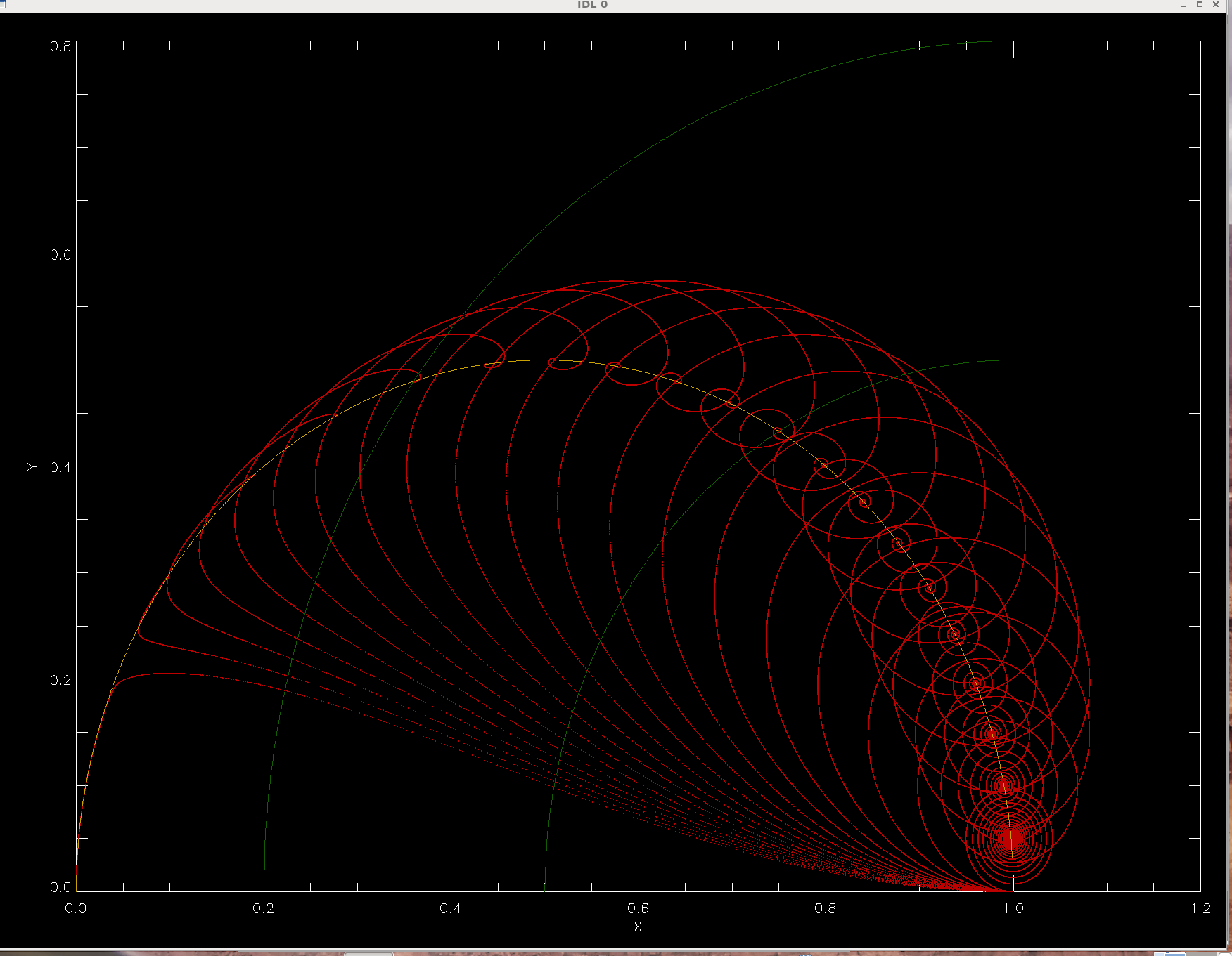
The higher the dog's speed s, the closer to the duck it eventually gets. For s=1, it reaches the duck in infinite time (and for s>1 in finite time). In every case, there is a fixed point to which the solution tends over the time of integration. Two green lines in the plot are circles drawn around the center of the pond (1,0), and have radii |R-1|=0.5 and 0.8 of the pond radius, for illustration of an important fact: the position of a (moving) dog with respect to (moving) duck tends to the radius equal s, as long as s is not larger than 1. You can see that two of the plotted trajectories (for s=0.5 and s=0.8) end at radius s.
We didn't have to do numerical solutions to find this fact, or even the precise
asymptotic positions. Fixed positions can be found analytically from the
evolution equations, as usual. Zeroing the r.h.s. we obtain R* (we'll skip the
* for simplicity, to avoid confusion with dot product or multiplication):
i(R-1) = s R/|R|.
Taking absolute value of this equation, we get |R-1| = s, precisely the point
we have noticed empirically; R-1 is the final position of the dog in the
rotating frame (dog enters a limit cycle that is a circle of radius s in
nonrotating plane). Now we've proven it. Notice that we can also prove it ad
absurdum: If |R-1| were not equal to s, the dog in its fixed position relative
to the duck would travel at a linear speed differing from s (their angular
speeds in fixed configuration being the same, the dog's linear speed is equal
to its radius |R-1|, but that number would be different from s). This is a
contradiction.
Furthermore, (R-1) as a vector is perpendicular to R, because the complex
numbers representing them differ by a factor i/s, which represents
rescaling by (1/s) and rotation by 90 degrees.
What is the locus of points such that vectors drawn from (0,0) and (1,0) to
those points are at right angle? It's a circle whose diameter joins the two
points, according to an ancient Greek geometry theorem. We can prove it by
writing the usual equation for the sought-after curve in terms of coordinates
x and y. We have R =(x,y), so the dot product of the two vectors R-1 and R
must vanish: (x-1,y)*(x,y) = 0. This can be written as either x(x-1) +
y2 = 0 or more familiar form of the equation of circle
(x -1/2)2 + y^2 = (1/2)2. This is such a valuable result
that we color half of this circle gold in our plots. So the fixed points are at
intersection of two circles with radii 0.5 and s, trailing the motion of the
duck by an angle θ = arccos(s). The family of solutions makes a beautiful
shell:

A final comment should be made about a visible change of behavior of those solutions which have a chance to approach the duck closely, i.e. for 0.9 < s < 1. The dog rushes towards the duck (lagging behind its circular motion by about 30 degrees), then slows down its approach to the duck's unit circle and turns sharply near the point M=(0.0504,0.2188) to either approach the duck very nearly along the golden path or alternatively turns RIGHT and swims toward its fixed point described above. The origin of the invisible magnet at M is totally enigmatic to your instructor, but then he hasn't read any of the historical literature on this problem cited by Strogatz. If anybody knows or can find out why the trajectories have a bifurcation near M, please let us all know during tutorial. The complicated shape of trajectories certainly prevented 19. century mathematicians from finding solutions to the problem in terms of elementary functions (they do not exist). However, a mystery remains. The fixed points are quite smoothly distributed along the golden bow, with density decreasing towards its left end for obvious reasons (according to arccos function describing the angle betweeen the duck, the dog, and the fixed point). They do not have any bifurcations or concentration points. They're oblivious to M, while the trajectories, especially the ones with dog's speed s≈0.97447, clearly are not and are ruled by something else.
In a way suggested in this graduate lecture: Carl Bender - Mathematical Physics 01 , we do something extremely strange, we indroduce a parameter $\epsilon$ where there was none before. By the way, that is not the only place where we can insert $\epsilon$, but first things first. $$ x^2 - \epsilon\, x - 4 = 0.$$ In perturbation theory, we usually expand the full solution in a power series of the parameter. After all, in NORMAL perturbation theories epsilon is small, therefore the convergence of series does not worry us. Let's suppose for a moment that what we are doing makes sense (even though we know we want later to substitute epsilon that is not at all small, $\epsilon=1$). $$ x= x_0 + x_1 \epsilon + x_2 \,\epsilon^2 + ...$$ OK, let's substitute this expansion into the quadratic equation and gather all the terms according to the power of the parameter: $$ x^2 -\epsilon x - 4 = [x_0^2-4] +[2 x_0 x_1 -x_0]\epsilon +[2x_0x_2 +x_1^2 -x_1]\epsilon^2 +O(\epsilon^3) \equiv 0 $$ To satisfy this equation for any $\epsilon$, all terms in square brakets must vanish. We list the parentheses multiplying consecutive powers of $\epsilon$: $$ x_0^2 - 4 = 0$$ $$ x_0( 2 x_1 - 1) = 0 $$ $$ 2x_0 x_2 +x_1^2 -x_1 = 0, \;\;\;\ etc.$$ Solving one by one, we obtain $x_0 = \pm 2$, $x_1 = \frac{1}{2}$, $x_2 = \pm \frac{1}{16}$, $x_3=...$
Now the risky step: not even knowing the radius of convergence of the series, let's risk it and substitute $\epsilon=1$, truncating the series to 3 first terms $$ x= \pm 2 + \frac{1}{2}\pm \frac{1}{16} = \{ 2.56250, -1.56250\}. $$ What is the EXACT solution? A quick algebra, which I managed to do a little wrong on the blacknoard :-| (thanks for correction!), gives $$ x_{exact} = \frac{1}{2}\pm \frac{1}{2}\sqrt{17} = \{2.56155, -1.56155\}. $$ This is different from our 3-terms perturbative solution by only 0.00105, a relative difference with the 2.56155 solution of only 0.00062(!). Our 3-term series returns exactly the same result as the 3-term expansion of the exact result: $$\frac{1}{2} \pm \frac{\sqrt{17}}{2} = \frac{1}{2} \pm \frac{1}{2} \sqrt{16(1+\frac{1}{16})} = \frac{1}{2} \pm 2 \sqrt{1+\frac{1}{16}} \approx \frac{1}{2} \pm 2 \pm \frac{1}{16} = \{ 2.56250, -1.56250\}.$$ Finally, let it be noted that no other place in the original equation benefits from introducing the $\epsilon$ parameter. Power series can be calculated but they diverge rapidly. Perturbations don't always work very well. See our textbook for examples of secular terms in time evolution of systems that should not have them (effect of resonance of higher-order perturbation terms with their driving terms, built from lower-order terms. But when they, work, they are fantastic. To increase the chance of correct placement of the the parameter in equation, always try to multiply the smallest term by the nominally small $\epsilon$. To know which term is the smallest, start by developing an idea of the approximate magnitude of solutions.
Richard Feynman developed a lot of perturbative series in the form of pictures called Feynman diagrams, in quantum electrodynamics.
x" = -3x/r3 +2 dy/dt +3x + b
(+ b stands for a constant, positive acceleration vector b along x-axis);
y" = -3y/r3 -2 dx/dt
where " is second derivative over time, b is rescaled β,
the ratio of forces of external radiation pressure and gravity of the object
located at the origin of coordinate system. Around the Earth, where radiation
is from the sun, b = βa/rL ~ 100 β = const.
(nondimensional radiation pressure to sun's gravity ratio).
First order perturbation theory can be applied to an initially slightly elliptic orbit (e≪1) of a satellite circling around a gravity center at (0,0) (the Earth), subject to a small acceleration b pointing along the x-axis (representing radiation pressure from the sun). Satellite's orbit lies in (x,y) plane and has instantaneous orbital elements a,e,w (a=semi-major axis, e = eccentricity, w = pericenter longitude, here defined as the angle between the negative y-axis and the direction to pericenter; variable w(t) should really be ω(t), but w looks similar and is easier to type).
Carl Friedrich Gauss at the end of the 18th century created a perturbation theory, from which today we can obtain the following evolution equations (2-d dynamical system) after time averaging over one period of the unperturbed orbit (in 1st order perturbation theory we evaluate the perturbation along an unperturbed, known trajectory, here - ellipse with semi-diameter a):
da/dt = 0
dw/dt = -β n (1-e2)1/2 sin(w)/e - np
de/dt = +β n (1-e2)1/2 cos(w)
where n, np, β = const.
[Explanation:
The perturbing force is given by nondimensional number β,
the mean angular speed of the satellite is n, and np is a precession
speed of the initial orbit due to frame rotation, if any.
A small rate of precession (np ≪ n) of satellite orbit is due to
the Coriolis force in (x,y) frame if it rotates. Why would it rotate? Imagine
that the (x,y) frame is attached to a planet that slowly orbits around a distant
sun, while the x-axis always points away from the sun (so it rotates in inertial
frame). The np is then the negative of angular speed of the planet.]
(i) If np is zero because the frame (x,y) is not rotating, solve
exactly the evolution of w and e as a function of time t, starting from
e0 = e(0) ≪ 1 and w0 = w(0) (arbitrary) at t=0.
Hint: Change variables to X = e cos(w), Y = e sin(w). Vector e=(X,Y) is
called Laplace-Runge-Lenz vector in celestial mechanics. Draw its evolution in
the orbital plane.
(ii) Additional question:
Explore the limit of e0 → 0.
The longitude of pericenter equation contains a term ~1/e, which is very large
initially; if e ≪ 1 then the evolution of w is much faster than the evolution
of e. Show that the system then becomes 1-D, and w adjusts to final value
instantaneously. Write the expressions for w(t) and e(t)
The diameter of the orbit (equal to 2a) is constant, but eccentricity can grow
to 1, which represents a needle-like orbit.
Demonstrate that the orbit becomes needle-like (e=1) and must collide with the
planet within a finite time; write an expression for the maximum survival time.
Try to solve the problem if np=const. is negative and small compared with n, but not zero. Is it possible to solve the Gauss perturbation equations analytically in that case?
The origin of terms in the equations is given on the blackboard (gravitational forces of two massive bodies, centrifugal and Coriolis forces). Click on the pictures:
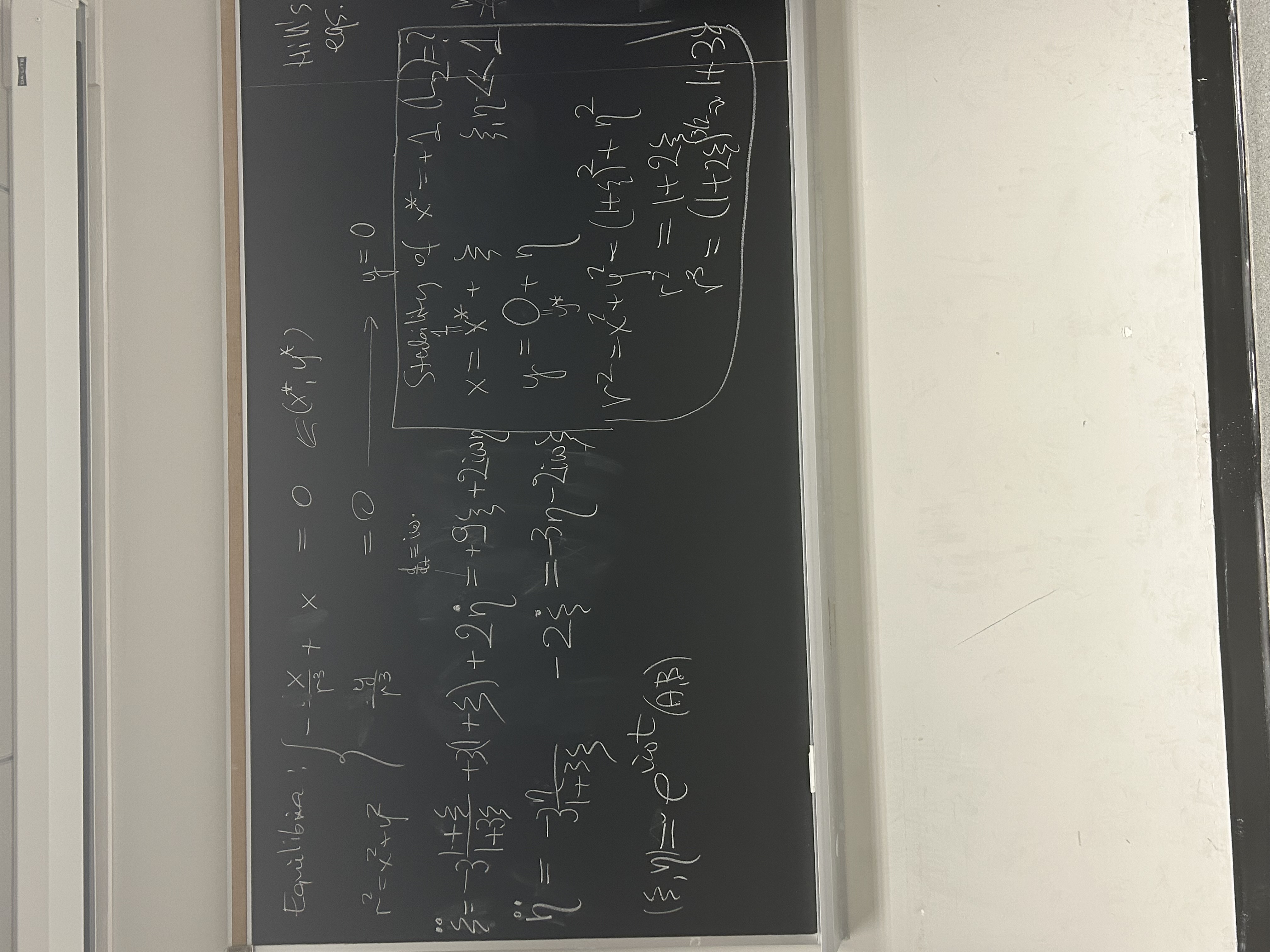
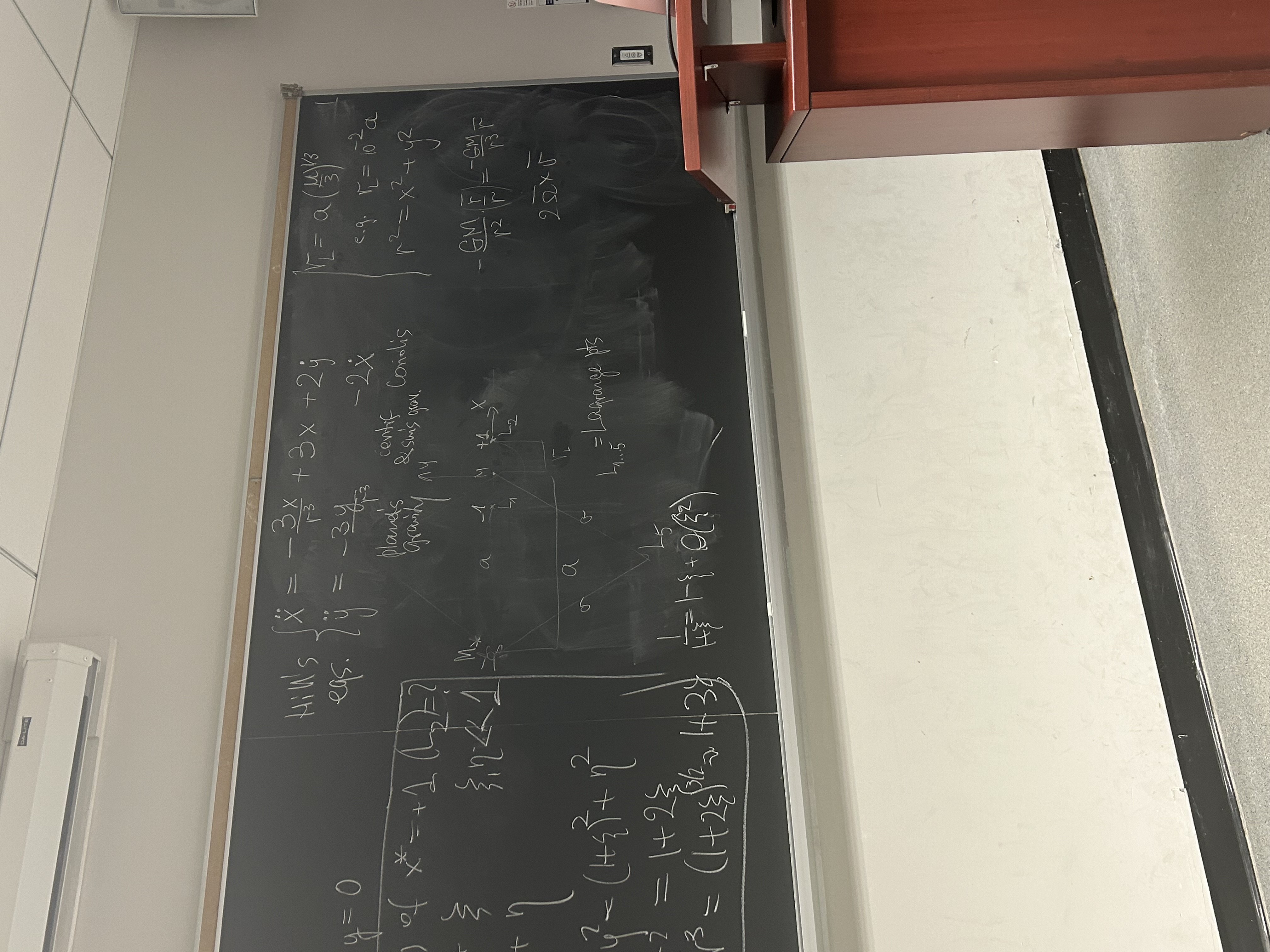
On the far right of the blackboard, you also see the typical way we write the gravity acceleration from a planet located at (0,0), using the usual dimensional distance r: -GMp r/r3. It is simply the absolute value of Newtonian acceleration GMp/r2 times the versor pointing toward the center of the planet, -r/r. After division by rL, the planet's gravity looks like -3r/r3 in the new nondimensional coordinate, confusingly also denoted by r. Number 3 comes from the cube of rL in the denominator (cf. the definition of rL above).
A native Sardinian, Giuseppe Luigi Lagrangia (better known as Joseph-Luis Lagrange, though he moved from Berlin to Paris aged 51 in 1787, so rather late in life), has found that the R3B problem has 5 equilibria/fixed points, places where a massless test particle can rest forever: 3 collinear with star and planet (L1-L3) and two in exact equilateral configuration with the massive bodies (L4, L5). Hills equations represent two of them, L1 and L2, while the other are too far away to be captured by the approximate form of equations. The scientifically important question is the stability of Lagrange points. Let's find out the distance to L2 (the same as to L1) from the planet's center, and then analyze the stability of the L-points.
As you see in the snaphots, L-points are found at (x*,y*)
= (±1,0). That is, L-points are indeed at the physical distance of
rL from the planet. Introducing small perturbations via:
(x,y) = (x*,y*) + (ξ,η),
we linearize the Hills equations, dropping terms of order
O(ξ2,η2) and higher, since by assumption they are
exceedingly small (even ξ,η ≪ 1). You can see that near the L-point
the y-component of restoring force is -3η but x-component has a repelling,
positive coefficient +9 in front of ξ. This is because L2, in common with
other collinear points, are saddles of the force field potential.
We seek solutions in the form (ξ,η) = (A,B) exp(iωt), where the frequency of oscillations ω in general can be a complex. If Im(ω) < 0 then the initially small deviations from the L-point grow exponentially in time and the point is dynamically unstable. Conversly, Im(ω) > 0 means Lyapunov stability (solutions stay close to the L-point forever).
I don't have a snapshot of the standard matrix analysis of the linearized equations. You will finish this job in assignments set 3, problem 3. One ω2 will be positive and the other negative. The existence of an imaginary frequency ω following from that means that L1 and L2 points are unconditionally unstable. The test particle will depart from these points upon the slightest perturbation. Despite that, it is precisely L2 where NASA and ESA have put their robotic observatories such as JWST and Planck, and sun-observing platform SOHO is near the L1 point! Why are these agencies not placing the spacecraft in the L4-L5 points, which are conditionally stable? (μ < 1/27 is neded for that, a requirement met by sun-Earth, and a lot of other binary systems).
The reason is that the triangular Lagrange points are maxima of effective potential. Too much fuel would have to be spent to climb the potential, in order to place objects there. (Incidentally, despite being maxima, these points are usually stable on account of strong Coriolis force, caused by frame rotation. This fictitious force bends the trajectories that try to roll down the effective potential and depart from the L4/L5 points, back toward them.) Meanwhile, L1 and L2 points are not only 100 times closer to Earth than L4 or L5, which is good for communication, their instability weak enough that it is corrected by occasional activation of thrusters on the spacecraft. It's one of the paradoxes of celestial mechanics: stable points are useless, while unstable points are useful.
If gas or particles are flowing through (the vicinity of) L1 or L2 Lagrange point, starting from rest or near-rest at the point itself and continuing inside or outside the Roche lobe of the smaller mass, the departure will be exponential in time, $\sim e^{\lambda t}$, with real and positive eigenvalue $\lambda$. Eigenvector associated with that value will be showing the direction of stream of matter. We want to know the angle that the vector forms with the horizontal axis (line connecting centers of massive bodies) in degrees, since there are some astronomical observations with which we can possibly compare our prediction.
We know that L1 point between the two massive bodies is an unstable
fixed point, located at $x_* = -1, y = 0$, when the equations of motion
are written in the formulation of Hill's problem as:
$$ \ddot{x} = -3\frac{x}{(x^2+y^2)^{3/2}} + 3x +2 \dot{y} $$
$$ \ddot{y} = -3\frac{y}{(x^2+y^2)^{3/2}} -2\dot{x} $$
Substitute $x= -1 + u e^{\lambda t}$ and $y = v e^{\lambda t}$ into the
equations: ($u,v$) is the constant eigenvector, and $\lambda$
its eigenvalue. The equations do not need to be turned into 4 first order
ODEs, though this would be a good method too. (But then you have to
deal with 4-dim. determinant.)
We just linearize the equations after substitution,
for instance this term
$$ -3x(x^2+y^2)^{-3/2} = -3(-1+u e^{\lambda t})[1 - 2 u e^{\lambda t}
+O(u^2,v^2)]^{-3/2} \simeq +3 +6 u e^{\lambda t}.$$
The linearized system, after simplification, has the form (cf. previous
topic, where linearized equations for L2 point were the same; we just
called $\lambda$ another name, $i \omega$):
$$ (-\lambda^2 +9) u + 2 \lambda v = 0 $$
$$ -2\lambda u + (-\lambda^2-3) v = 0.$$
Notice that we have already seen those +9 and -3 force coefficients
(curvatures of potential at L1,2 points) before, in the previous topic.
No wonder - it's the same set of Hill's equations, there around L2 and
here around a mirror-reflection L1 point.
Determinant of the matrix is zero when
$$ (9-\lambda^2)(-3-\lambda^2) +4 \lambda^2 = 0$$
This characteristic equation is bi-quadratic, $\lambda^4-2\lambda^2-27=0$,
and has the following solutions: $\lambda^2 = 1 \pm 2\sqrt{7} $.
One of the four solutions is real and positive, $\lambda_+ =
(1+2\sqrt{7})^{1/2} = \sqrt{6.2915} = 2.5083$.
That is the inverse timescale of e-fold growth of distance from L1
(exponential timescale of instability).
Meanwhile, the associated eignevector coordinates satisfy both matrix equations (we take the first eq.) $$ (9-\lambda_+^2)\, u + 2\lambda_+\,v = 0.$$ Taking $u=1$ we get the eigenvector (1,-0.5399), but if we want the direction of flow in reverse direction, $u=-1$ and the vecotr is (-1,0.5399). The inclination $\phi$ of eigenvector to horizontal axis satisfies the relationship: $\tan \phi = v/u = (\lambda_+-9\lambda_+^{-1})/2$, thus $$\phi = \mbox{arctan} (-0.53989) = -0.49506\, \mbox{rad} = -28.365^\circ$$ This direction of flow is valid for all binary systems with small secondaries, which is the assumption of Hill's problem, but does not depend on exactly how small the mass ratio is, or in which of the two colinear eigen-directions the matter is flowing from the L1 point (corresponding to two possible donors of mass, primary and secondary component of the system). The nondimensional time of $\Delta t = 2\pi$ is the full rotation of the binary system. In this time interval, the initially very small separation from L1 point grows by a very large factor $\exp (\lambda_+ \Delta t) \simeq 7 \cdot 10^{6}$.
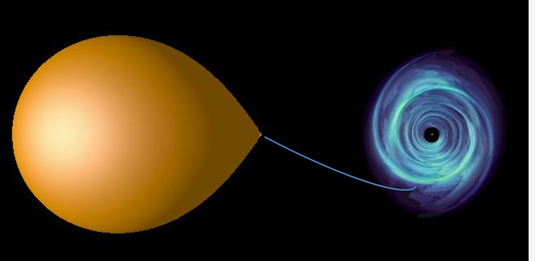 This clickable image schematically shows the shape of the stream
(which wasn't modeled in this CFD=comp. fluid dynamics simulation, but it
could have been..) Notice that the mass ratio in this circular R3B problem
wasn't small, and the R3B rather the local Hill's problem was modelled.
Therefore, there are at least 2 reasons not to compare the angle of stream
in the picture with 28.36$^\circ$: 1. mass ratio is not small, 2. I added the
stream using Powerpoint :-). Having said that, for one reason or another
the angle in the picture is about 30$^\circ$.
This clickable image schematically shows the shape of the stream
(which wasn't modeled in this CFD=comp. fluid dynamics simulation, but it
could have been..) Notice that the mass ratio in this circular R3B problem
wasn't small, and the R3B rather the local Hill's problem was modelled.
Therefore, there are at least 2 reasons not to compare the angle of stream
in the picture with 28.36$^\circ$: 1. mass ratio is not small, 2. I added the
stream using Powerpoint :-). Having said that, for one reason or another
the angle in the picture is about 30$^\circ$.
You will have the opportunity to numerically study the trajectory emanating from L2 point in one of the assignments. Then you can see what happens with the stream later on, assuming it can self-intersect.
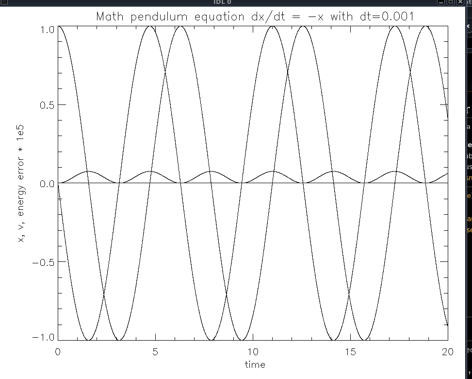
The second method we explored was perturbation theory. We noted that if we start very near the fixed point, the amplitude of oscillations is small, and the amplitude of vq is small or even much smaller, if q > 1. Thus we can treat the power of v as a small addition to the periodic solution of s" = s(1-s2) equation linearized around the (s*,v*)=(1,0) fixed point, which reads x" = -2x, when we denote x=s-s*. The linear solution is a sinusoidal function of time with angular frequency ω = √2. Linear equation has energy E = ½(ds/dt)2 +½ω x2 = const. To find out the addition to this energy in time equal one period of the orbit, we integrate from 0 to full time period the product of the perturbation to acceleration (or force) multiplied by v, here -vq+1. This is so because force component along the velocity vector times (dot product) velocity vector in physics is power, or the rate of change of energy E. Since v does small harmonic oscillations around zero and for even q the term vq+1 is an odd function of time, the integral expressing ΔE is zero and the energy after a full circle in phase space is unchanged. Physically speaking, on half of a circle perturbation adds energy, and on the rest it removes an equal amount.
Not so if q is odd: the power of perturbation, (-vq)v, stays negative and steadily saps energy out of the system's oscillations, making them die exponentially fast. We see this in the decay of amplitude in numerical results above.
Scripts from tutorial that you can freely use:
You can for instance use the ideas from the scripts and re-write them in
Python or Matlab or C. The IDL script is a template but not a final program that
you need, so don't copy it mindlessly - it might not do what you want to do,
have inefficiencies etc. The computational kernel in it was verified though, and
that's what you want to use.
In tutorial 8 we study the integration schemes of 2nd order Euler-like, and Leapfrog (Verlet) method. I used IDL (interactive data language) scripts that also run under GDL (free IDL), and you are encouraged to rewrite them in Python, Mathematica, Maple, Matlab or Octave (free Matlab replacement), Fortran 77 or Fortran 90/95/2003 (great language for number crunching), Julia, Haskell, or C/C++ . The re-writing is a good idea, as the skills you gain while doing it will be very useful for you outside this course.
inte1.pro,
inte2.pro
inte2.png
(results of inte2.pro)
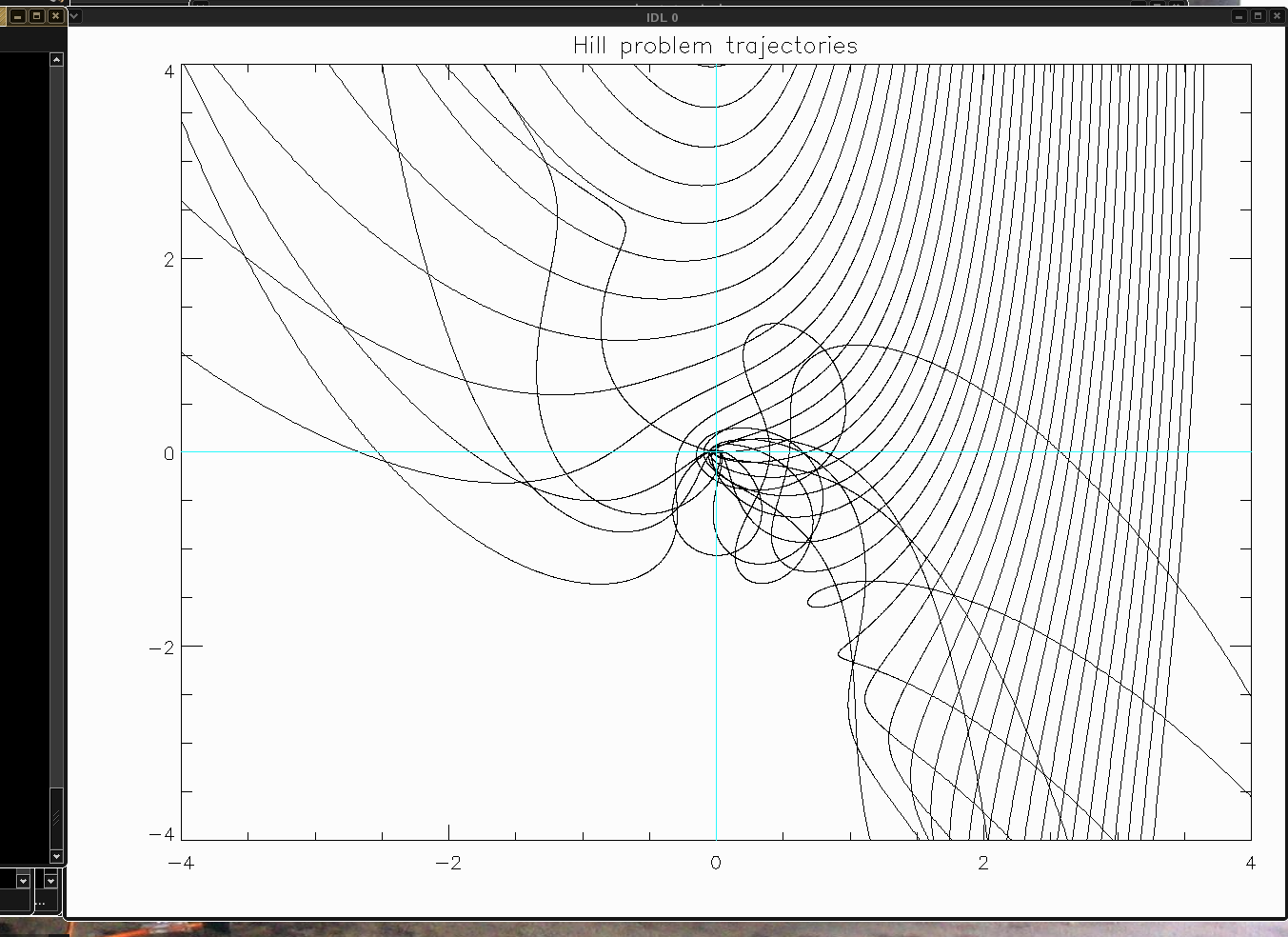

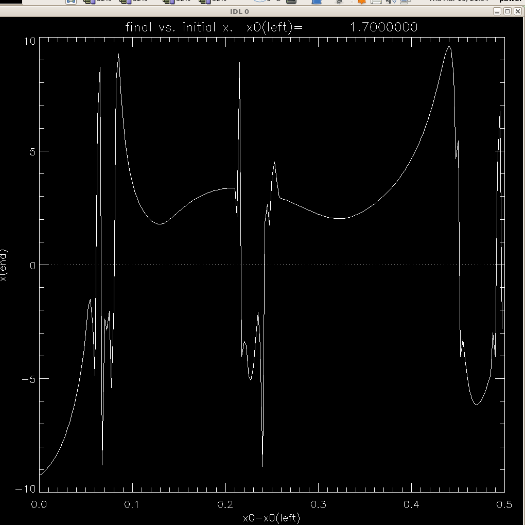
Program hill3.pro . Solves Hill's problem
for a range of starting positions outside the orbit of the planet (positive
radial coordinate x). Vertical motions are neglected, but you can add the
z-equation to the system, the only z-force is from the planet.
We start by identifying larger scale features
x-y view of orbits (units are Hill sphere radii) , and the corresponding
graph of
function x(x0) . Not clear if it's chaos. To establish chaos strictly, we'd
need to evaluate and plot the Lyapunov exponents at different x0's.
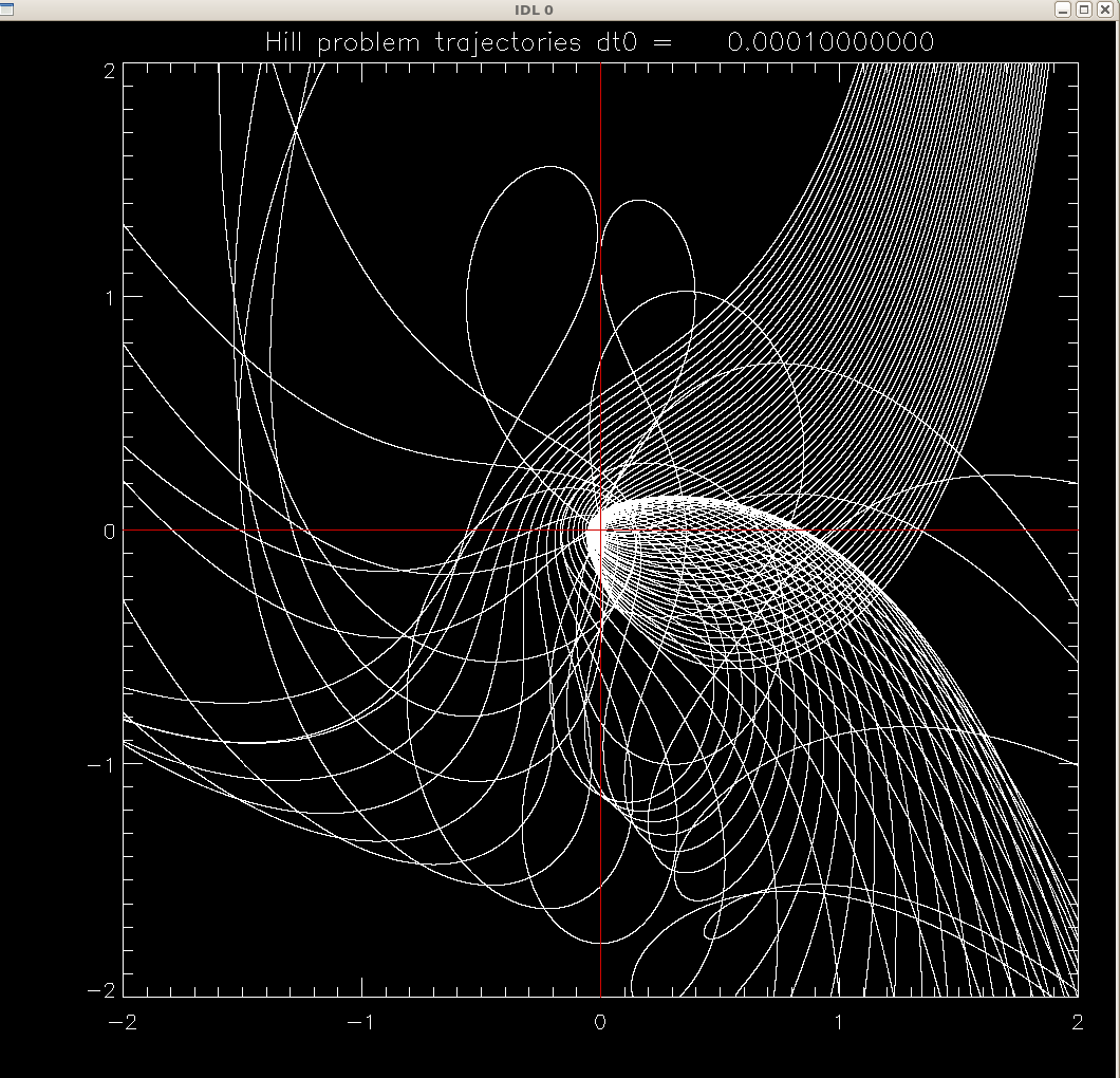
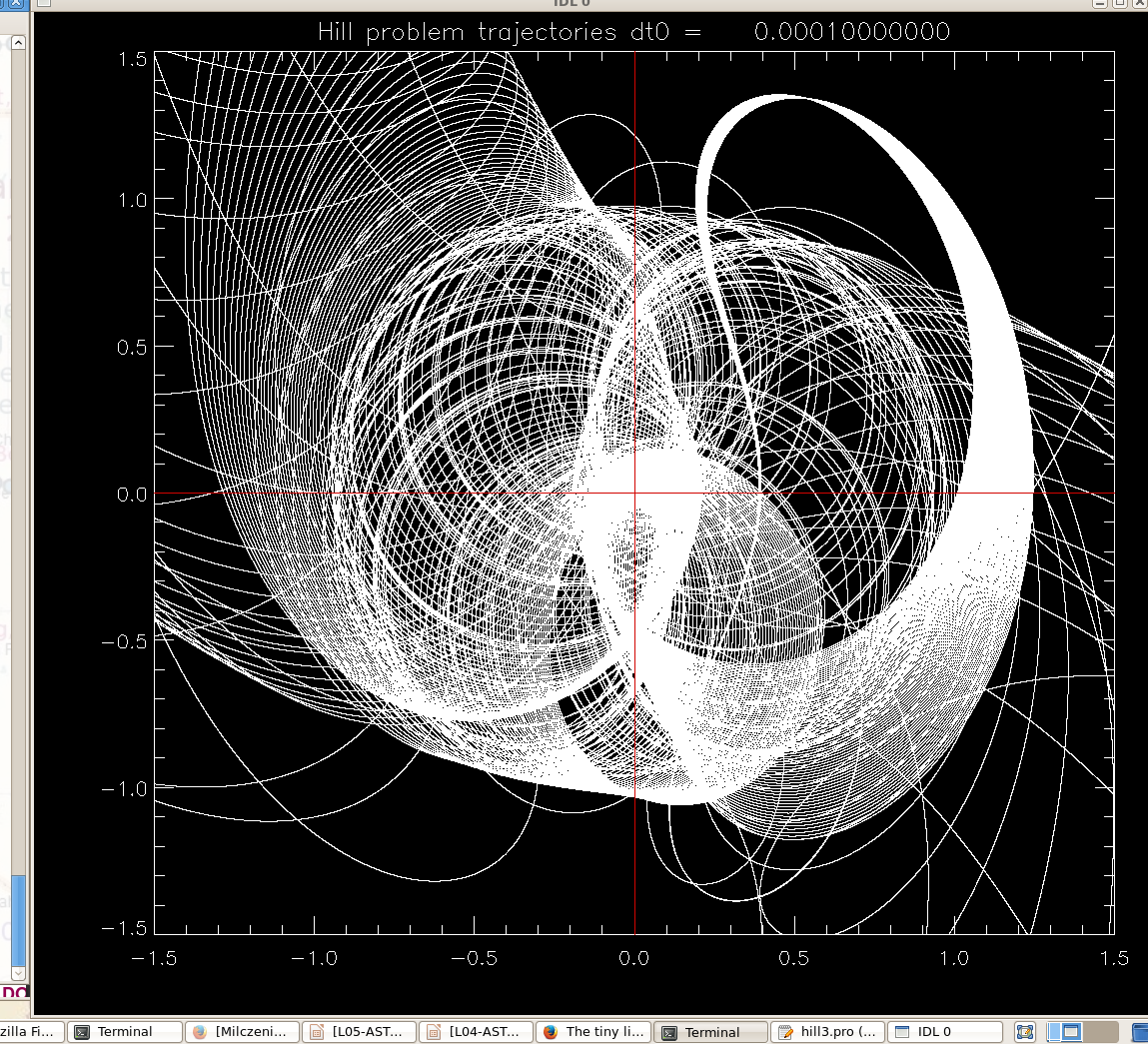
Or one can start zooming in ... but there does not seem to be a self-similarity
in the graphs, it's a complicated system that may not have self-similarity,
even though arbitrarily close starting conditions often diverge into different
outcomes, and in that sense the system is chaotic and the set leading to
a given outcome (say, switching from positive initial x to negative x at the
end) is likely a fractal.

A very nonlinear 4-d dynamical system (two angles and two angular speeds):
not only the trigonometric functions contain all possible powers of angles, but
they are inside rational functions (fractions)


Animation of N ≫ 1 pendulums, in initially similar states. It looks like initial speeds were the same (zero) but initial angle(s) were differrent from 0.01 to 0.0001 radians.
en.wikipedia.org/wiki/Double_pendulum tells more about the double pendulum, and shows a connection to fractals. Namely, in the plane of two starting angles, there is a region that never results in rotation of the lower arm (sure, if the angles are small energy is not sufficient). But the region is not a simply connected area, it's a fractal. Take a look.
xn+1 = e-b xn2 + c
gauss-map-4.6.pro , gauss-map-9.pro , gauss-map-4.6.pro
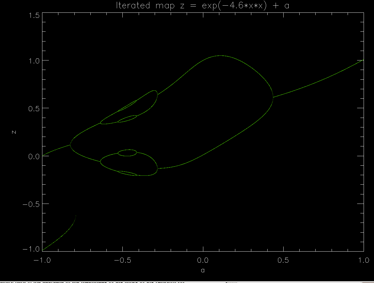
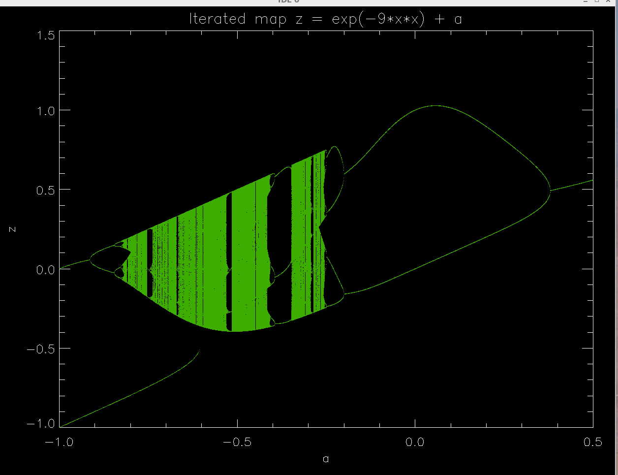
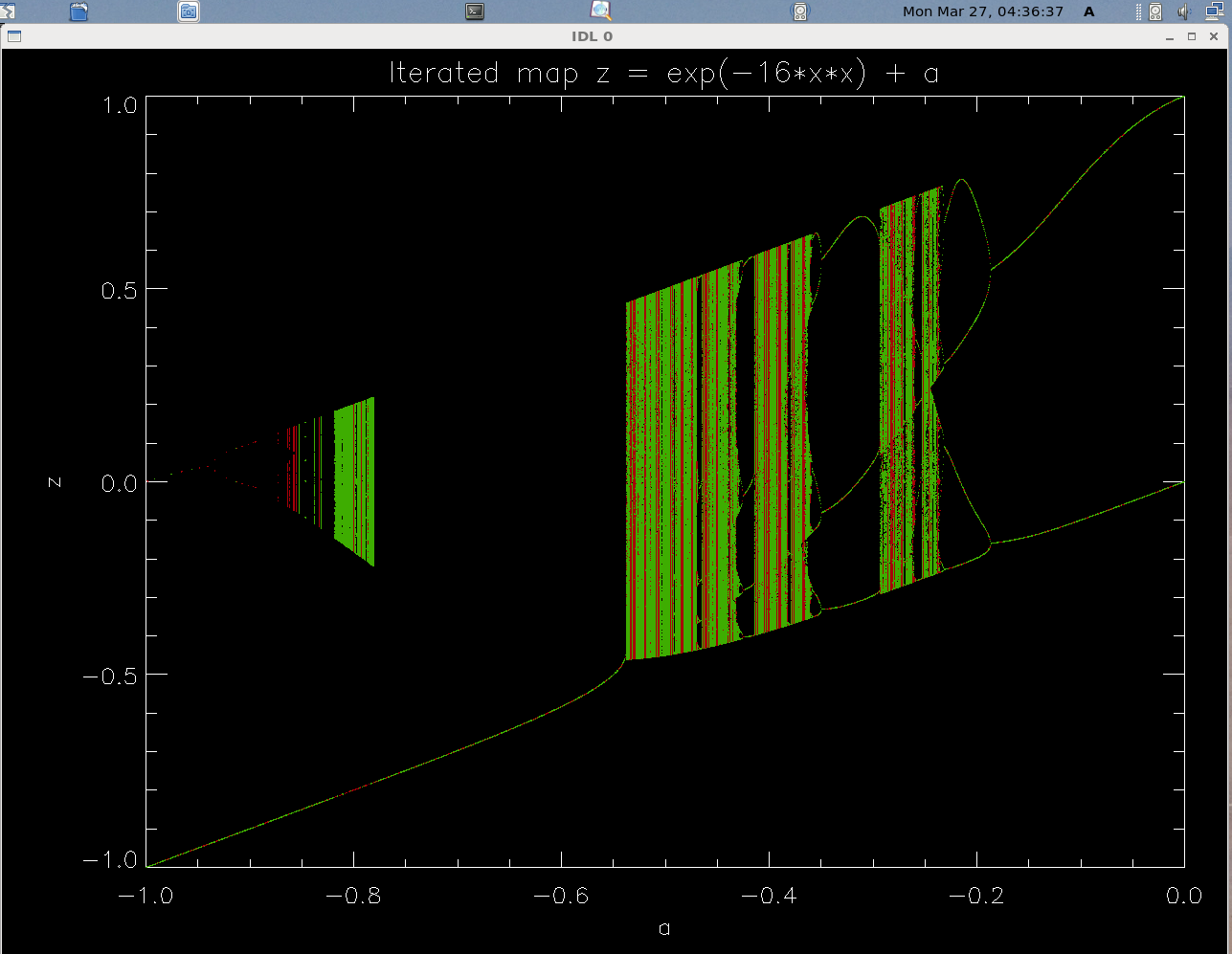
Notice that parameter b controls the steepness of the slope of the gaussian curve, and therefore the number of places in which a diagonal line in a spider diagram can intersect it.
In the last picture, b=16 is so large that we get two separate regions of chaotic behavior -- I believe that the space inbewteen is in fact empty not because the starting value of the variable is incorrectly chosen. I have a line in the appropriate version of the script (see above) which randomizes the starting point in a fairly wide range.
θn+1 = θn + Ω + (K/2π) sin θn
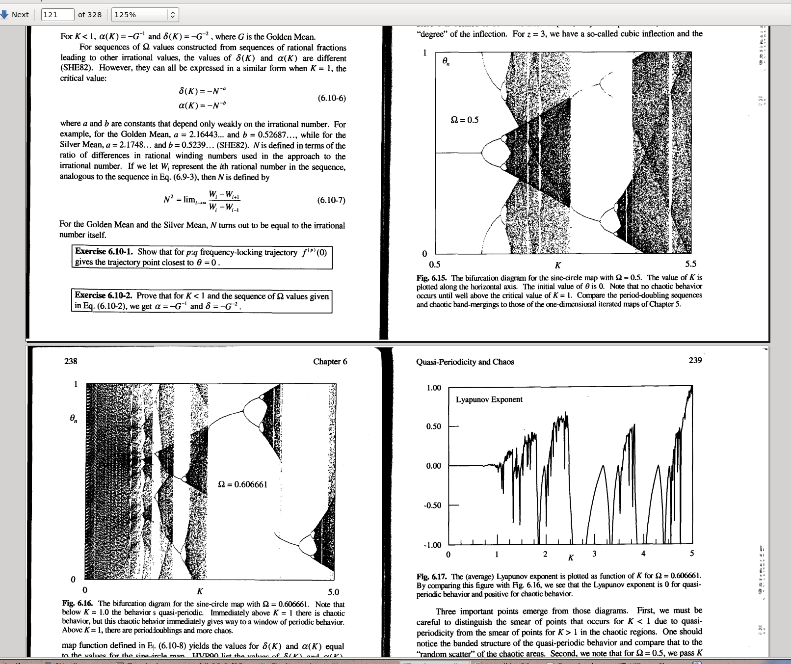
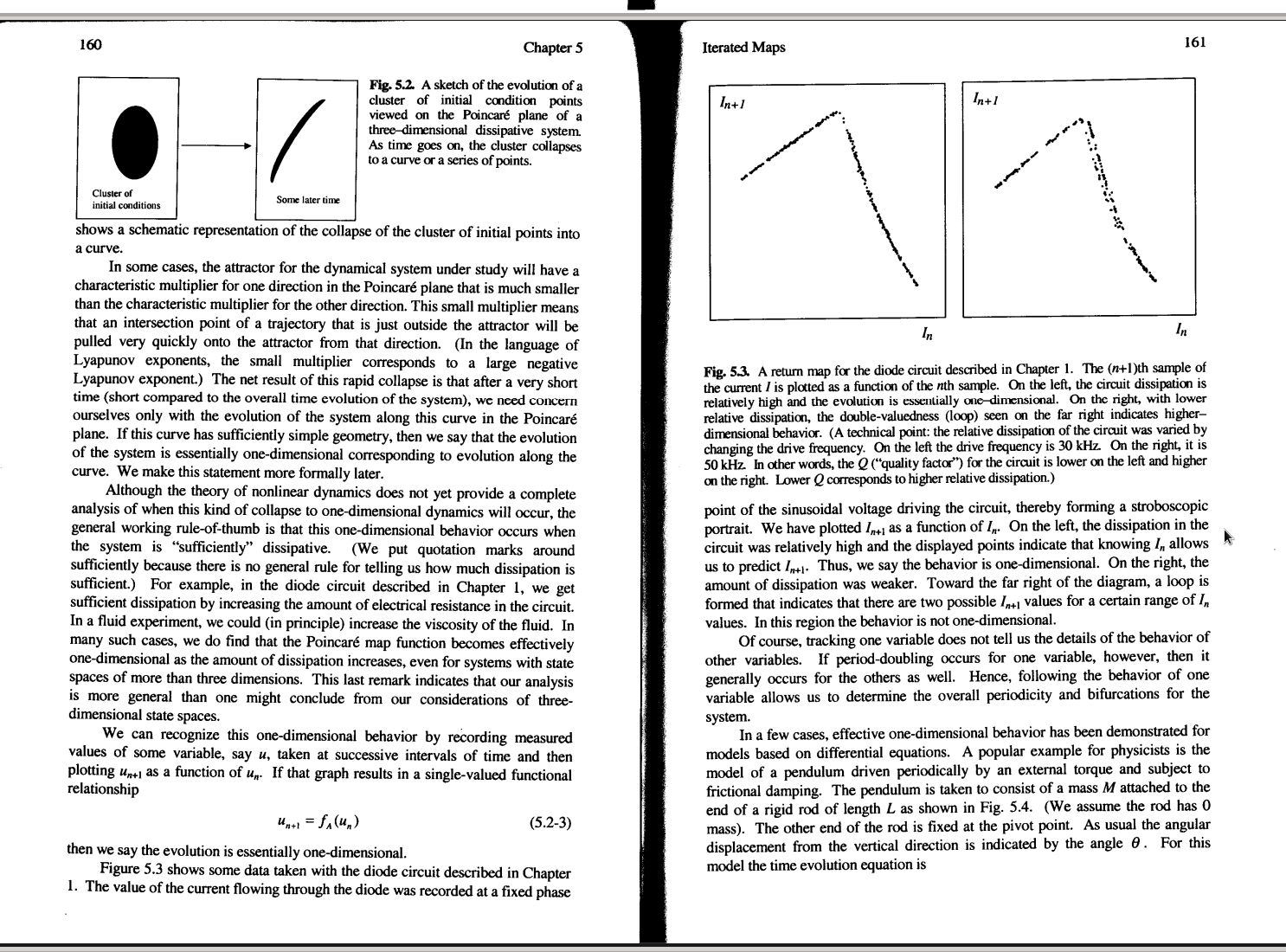
From Robert Hilborn's book "Chaos and Nonlin. Dynamics" 2ed 1985 (CUP). Pages: 9-18, 161

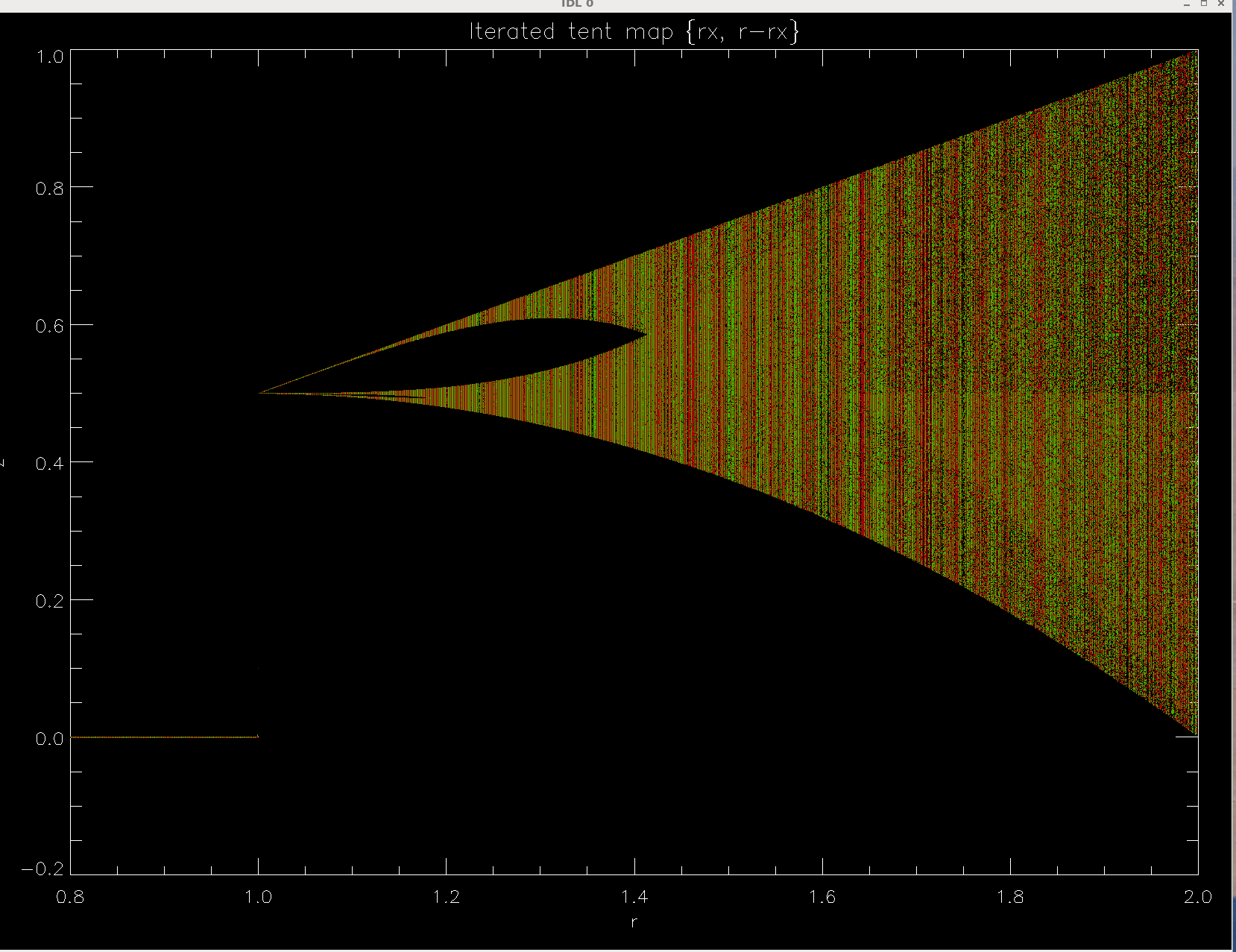
tent-map.pro,
tent-map-zoom.pro.
 and this picture
  that clarifies why we call parts of Mandelbrot set n=1 continent, n=2
continent and so on.
that clarifies why we call parts of Mandelbrot set n=1 continent, n=2
continent and so on.
See this video introducing turbulence,
Fluid dynamics is complicated because, unlike many parts of physics, it is
intrinsically nonlinear (with exception of classial acoustics, which treats
sound waves as weak perturbations, and uses linearization)
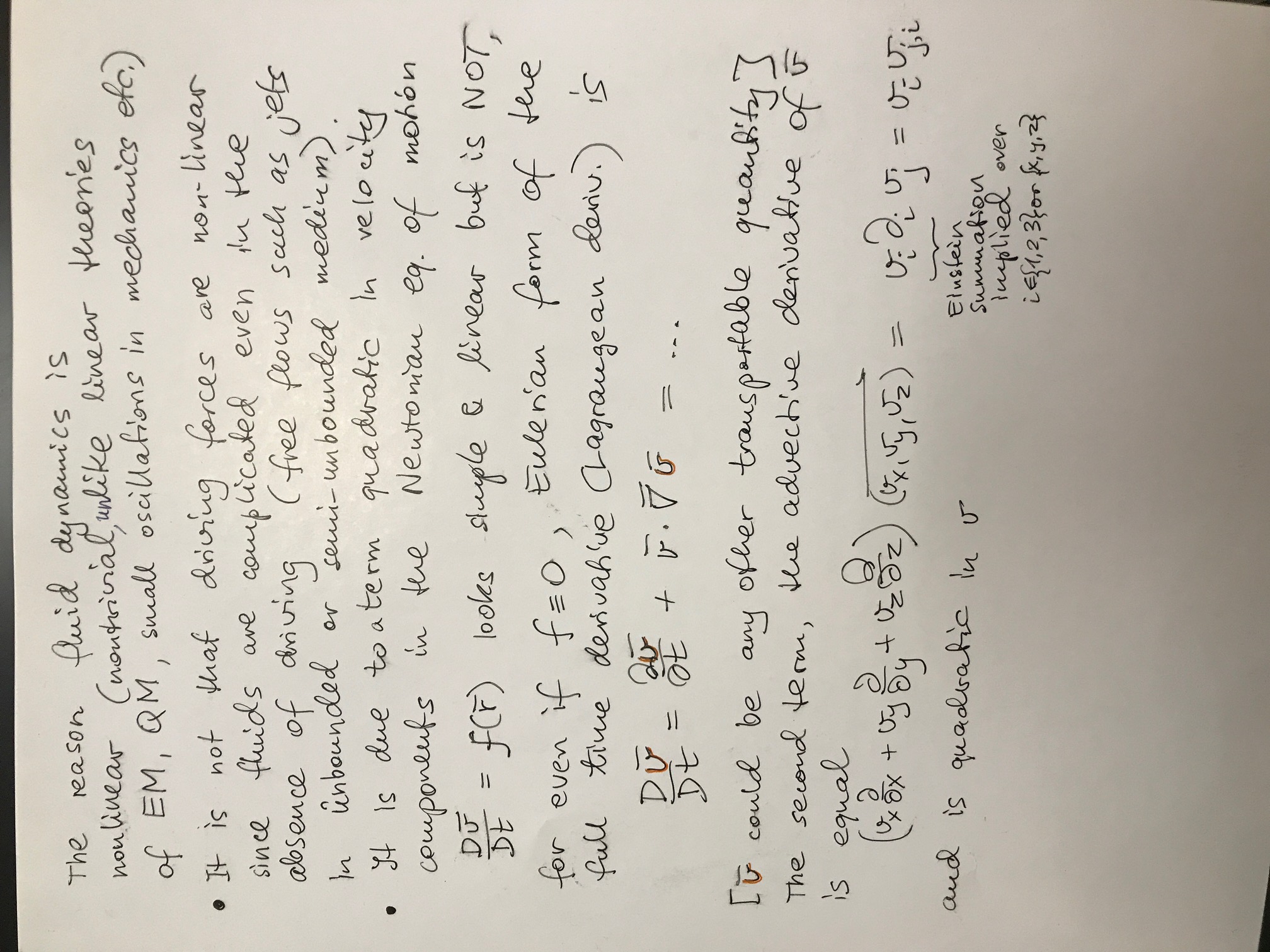
Lack of superposition principle makes some hydrodynamical problems difficult. Enough so that Werner Heisenberg (story of Heisenberg's PhD in hydrodynamics) supposedly said that when he meets God he'll ask two questions, "Why quantum mechanics?" and "Why turbulence?”, and that God will have a good answer to the first question (more about fluids here).
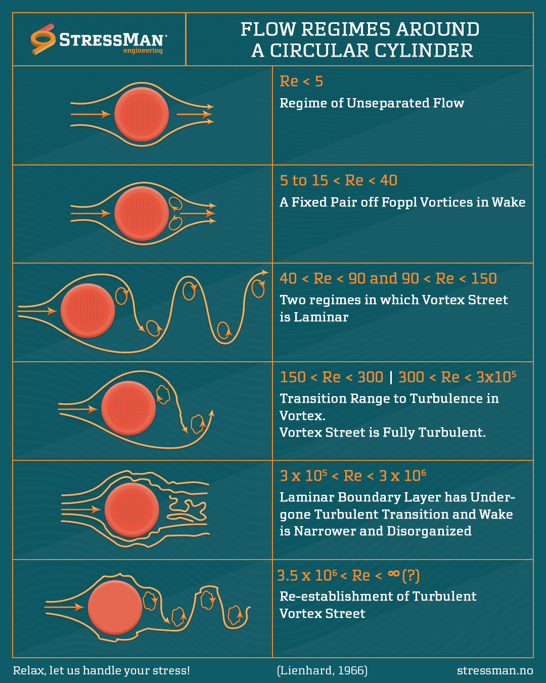
But some people loved it. In the beginning of 20th century, Theodore von Karman
as a graduate student helped his office-mate in his PhD studies. The other
student (Karl Hiementz) was tasked by a leading German aerodynamicist Ludwig Prandtl with
experimentally measuring a steady wake behind a cylinder (like a bridge support
in a streaming river), but could not obtain a steady flow no matter how much he
perfected the experiment, getting really worried. It was a relief when von
Karman proved that cyliders and other shapes do not produce steady wakes
under nomal conditions. Instead, they periodically shed alternately rotating
vortices, which form a stable configuration in the wake - a von Karman vortex
street. Even a sphere, whose symmetry would not logically single out any planar
arrangement, does something
like this.
It's like a bifurcation from a stable node to a period-2 cycle. At higher flow
speeds, further period doublings and eventually chaos abruptly happens. We call
that chaos fluid turbulence.
Later, von Karman explained why Tacoma bridge collapsed in 1940: it was very slender and its twisting/bending modes were in resonance with the frequency of von Karman vortex shedding! It took a decade to convince professional architect societies that something as heavy and tough as a steel bridge can be destroyed just because air is flowing around it. Not a hurricane, just a strong wind. Architects started paying attention to aerodynamics and aeroelasticity (how an elastic body interacts with the air flow) and through progress in CFD (computational fluid dynamics), today our bridges and buildings do not collapse (because of wind). See, however, a fascinating and scary story about one famous high-rise building in NYC that was secretly reinforced, because it COULD have collapsed, causing sort-of domino effect (wiki article).
As to the turbulent jets, we need to have a degree of control over their chaos.
Sometimes not to decrease it but to enhance it. For instance, efficient burning
of fuel that minimizes emission of harmful nitrogen and carbon compounds,
requires very good mixing of fuel into the stream of air, to be
injected into cylinders.
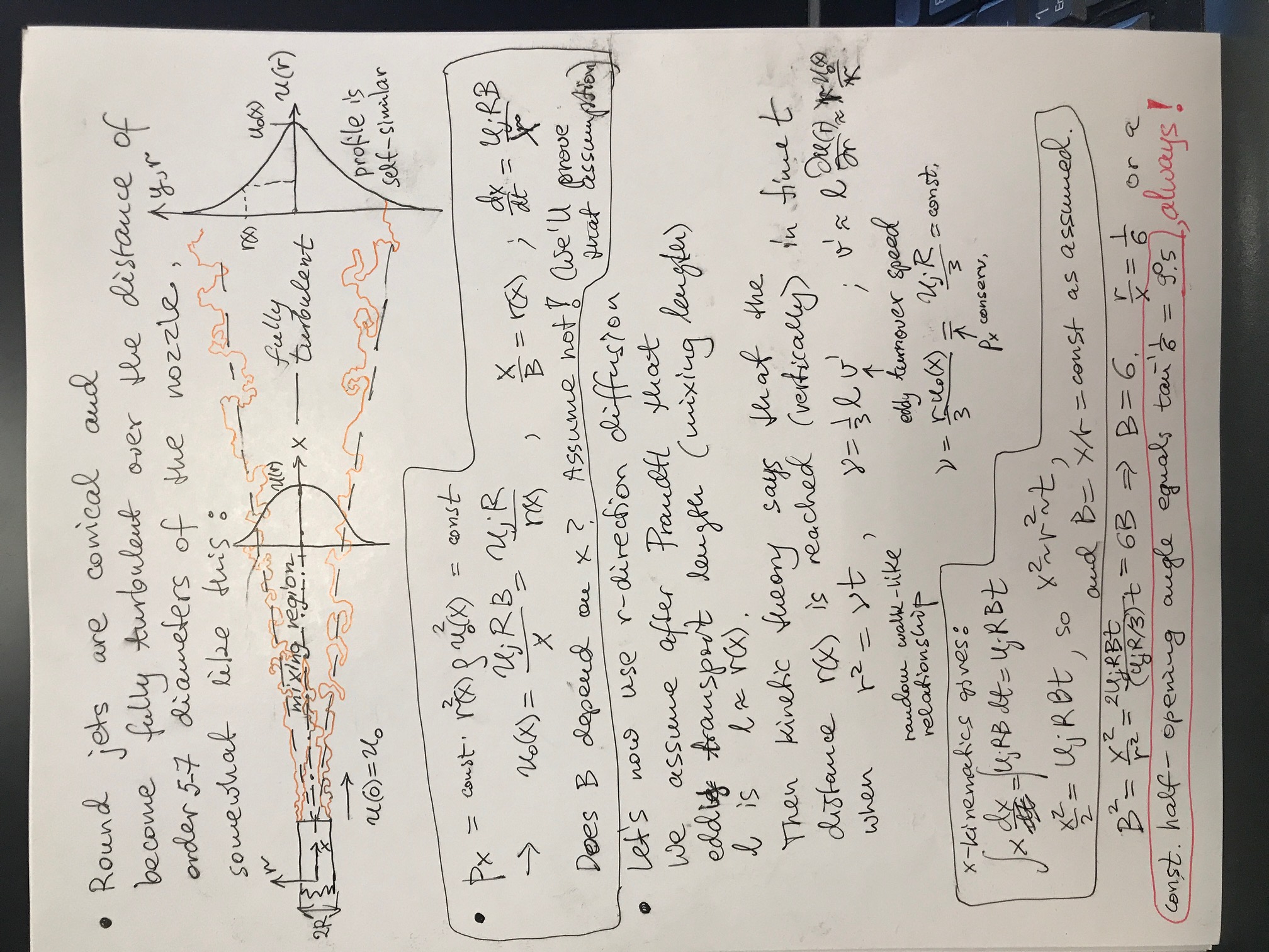
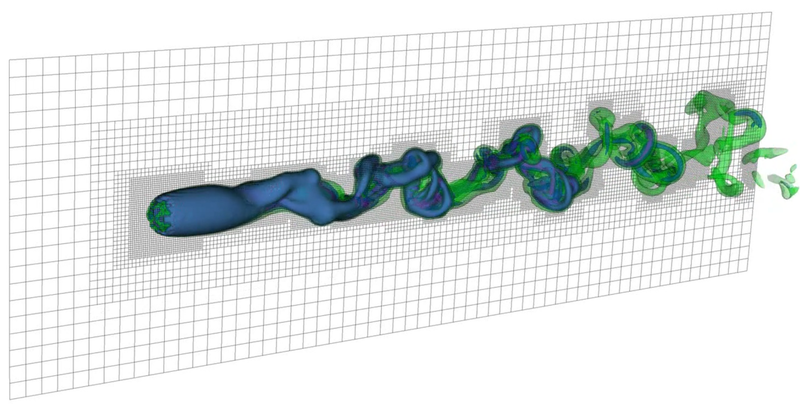
Animation of jet
simulation with DNS method (direct numerical simulation of Navier-Stokes
equations describing fuild's motion), on a 0.6 billion points 2-D mesh. It shows
the mixing region where ring-type instability first operates and later something
like a von Karman vortex stret is seen along the edge of the stagnant,
surrounding fluid. Jet flow gradually loses laminarity and becomes fully
turbulent at distances exceeding 5-7 nozzle diameters. (That's a rule, no matter
whether it's air or water, or two similarly dense gases or liquids, and
independent of jet speed, turbulence manages to establish itself before the flow
reached 10 muzzle diameters, after which the jet is a cone, and its profiles of
speed as a function of perpendicular distance (radius) become self-similar.
See some commonly observed facts about turbulent jets in this lecture notes file:
https://cushman.host.dartmouth.edu/courses/engs250/Jets.pdf
Further theory is provided by this monograph by S. Pope titled simply Turbulent Flows ; see pp. 111-122.
We will heuristically prove that all turbulent jets into stationary environment have full opening angle slightly less than 20o. For this, one splits the flow into the bulk flow part and turbulent fluctuating part. Eddies have a preferred scale (called mixing length) and rotate at a speed adjusted to the gradient of velocity in the underlying jet. Momentum of the fluid in x-direction (along jet) is approximately conserved, from which it follows that the velocity near the central peak of speed of the flow falls with distance as 1/x. The sideways diffusion laws are also known and result in the forumula for mean-square distance travelled in time t, in the form r2 = ν t, a relationship also common in random walk, diffusion of tracer chemicals in still air, and many other diffusion processes. Together, r- and x-motion provide a formula for half-thickness of a round jet at distance x from the nozzle: r(x)= x/B, where B is a pure number equal to 6. Full opening angle of jet's cone is 2 atan(1/B) = 19°.
There are many applications for the knowledge of turbulent jets. Now you understand that there is a beautiful self-similarity, manifesting itself as a universal constant, the opening angle of a turbulent jet ≈ 20 degrees (full angle), if the jet enters a stationary air or water -- what enters what is unimportant, as long as there is no big density difference, which might affect the mixing. But temperature difference is not important, at least in horizontal flows, since in the vertical direction it produces force of buoyancy, which may stop or accelerate the jet's motion.
Let's take a jet or recirculated water entering a swimming pool. Next time you are in the pool, feel with your hands under the surface the relatively well defined, pulsating (due to intermittency) boundary of the jet. Estimate the cone angle. In fact the jet can be visualized dramatically with food coloring. If it's not your pool, you won't be very popular afterwards. Another way to visualize water jet is to somehow introduce small air bubbles into it.
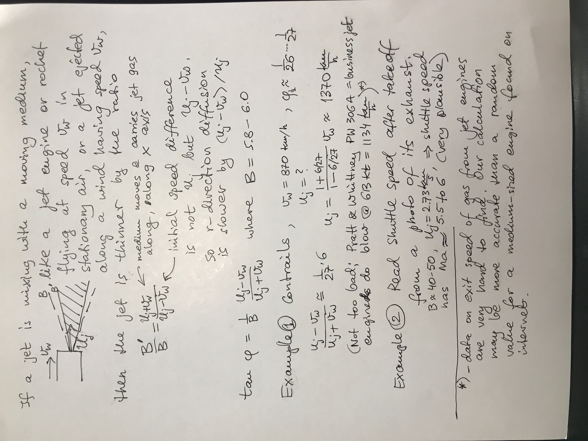
Next application is the condensation trails of high-flying airplanes. What you
see is not chemical polutants or 'chemtrails' of conspiracy theories. It's
condensed water from the exhaust. Ideal burning of fuel produces just water and
CO2. Rockets, especially solid fuel boosters, leave a more polluting
type of smoke in their exhaust. From snapshots of their trailing jets we can
estimate the momentary speed of the object (we have to know the nozzle speed
for that).
See the following modification of the theory to handle the nonzero ambient
medium speed, and two sample applications:
The first part of this lecture 23/24 has the same details as above, plus the story of some nonlinear phenomena from astrophysics of planet formation, with surprising appearence of our old acquaintances: pitchfork and imperfect pitchfork bifurcations.
Here is the proof of the superstable nature of this discrete map representing the method $$ x_{n+1} = f(x_n) = x_n - \frac{g(x_n)}{g'(x_n)}. $$ The iteration converges to $x_*$, the zero of function $g$, i.e. $g(x_*) = 0$. So we consider deviations $\epsilon$ from that zero: $ x_n = x_* + \epsilon_n$. $$ x_{n+1} = x_* + \epsilon_{n+1} = f(x_* + \epsilon_n) = f(x_*) + f'(x_*) \epsilon + f^"(x_*)\frac{\epsilon_n^2}{2!} + O(\epsilon_n^3). $$ Subtracting $x_* = f(x_*)$ from both sides, $$ \epsilon_{n+1} = f'(x_*)\epsilon_n +f^"(x_*)\frac{\epsilon_n^2}{2!}+ O(\epsilon^3).$$ Let's calculate those derivatives of $f(x) = x-g(x)/g'(x)$. They need to be evaluated at $x=x_*$, where $g=0$, which we do in the last equality of each formula: $$ f'(x) = 1 -\frac{g'}{g'} +\frac{g \,g^{"}}{g^{'2}} = \frac{g \,g^{"}}{g^{'2}} \;\;\stackrel{x_*}{=} 0$$ $$ f^"(x) = \frac{g^" }{g'} +\frac{g\,g'''}{g'^2} -2\frac{g\,g^{"2}}{{g'}^3} \;\;\stackrel{x_*}{=} \frac{g^"(x_*)}{g'(x_*)} $$ Substituting into the $\epsilon_{n+1}$ formula, and dropping small higher-order terms $O(\epsilon^3)$, we get $$ \epsilon_{n+1} = \frac{g^"(x_*)}{2 g'(x_*)} \,\epsilon_n^2.$$ This equation says that from the step in the iteration in which the error $\epsilon_n\approx 0.1$, each step of the iteration doubles not the accuracy but the number of accurate decimal digits. This a fantastically fast convergence to the root of equation $g(x)=0$. Deviations $\epsilon_n$ shrink like $10^{-1}, 10^{-2}, 10^{-4}, 10^{-8}, 10^{-16} ...$ but beyond that, a normal math software fails to represent or operate on the number of accurate digits larger than 16. So you get a double precision accuracy after 5 or so iterations. Convergence is faster than exponential. We call such a fixed point (and the convergence to it) superstable.
Caveat: If the starting point $x_0$ is chosen too far from $x_*$, then the Newton's iteration can go very wrong, one example of which we saw by doing a graph of a complicated function with many local maxima. In fact, if the function $g(x)$ has singularities or compact support, i.e. is not defined for all real $x$, then there is no guarantee that $x_n$ is in the domain of the function. The iteration may fail.
Comment: If, on the other hand, one devises some approximation that allows to start the iteration from an already small error $\epsilon_0 \approx 0.001$, then one reaches a single precision accuracy for the root in just one iteration. This is actually used in some PDE/CFD algorithms, which need to numerically solve for a zero of some function in each spatial cell. To save time, they do it in one iteration, starting from a value obtained in the preceding time step.
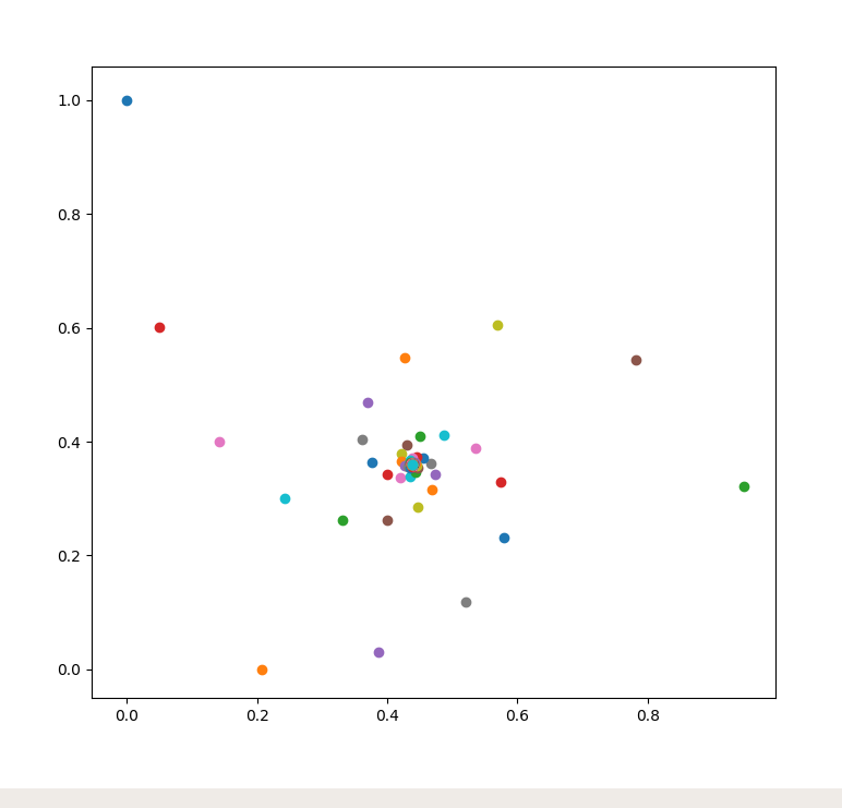
Using expansion $i = \exp i \pi/2$, and the rule $(a^b)^c = a^{bc}$, in the tutorial we have found that $i^i$ is in fact a real number equal to $e^{-\pi/2} \approx 0.207$. When you raise $i$ to that number, however, you get a complex number. The iteration $z_{n+1} = i^{z_n}$ proceeds further, returning complex numbers, which converge in a 3-armed spiral way toward $i_\infty$ that represents some new mathematical constant with unknown relationship to any other mathematical constants such as $e$, $\sqrt{2}$, or $\pi$.
In order to iterate any map (in this case, the self-exponentiation), we wrote
this little
script called iter_expo.py, which created this clickable illustration
of the $z_n$ series.
and printed
$ python3 iter_expo.py
0 1j
1 (0.20787957635076193+0j)
2 (0.9471589980723784+0.32076444997930853j)
3 (0.05009223610932119+0.6021165270360038j)
4 (0.387166181086115+0.030527081605484487j)
5 (0.78227568243395330+0.5446065576579896j)
6 (0.14256182316366683+0.4004665253370873j)
7 (0.5197863964078542+0.11838419641581431j)
8 (0.56858861727189700+0.6050784067978037j)
9 (0.24236524682521116+0.30115059207131784j)
10 (0.5784886833771008+0.23152973530683355j)
11 (0.42734013269162796+0.5482312173435612j)
(...)
94 (0.4382932210669228+0.36059975439717595j)
95 (0.43827209785842985+0.3605954271051038j)
96 (0.43828704142255887+0.3605833359079871j)
97 (0.43828690144249010+0.3606004726004544j)
98 (0.43827518297007520+0.3605906696281181j)
99 (0.43828856933122223+0.3605881545537939j)
(...)
335 (0.43828293672703206+0.3605924718713856j)
336 (0.43828293672703200+0.3605924718713853j)
337 (0.43828293672703230+0.3605924718713855j)
(...)
335 iterations are needed for $z_n$ to approach $z_\infty$ to within 15 digit accuracy. If you are ever faced with a convergence of a series that you want to accelerate, know that there are techniques to extract from a given series a much more accurate (faster converging) series.
In our case, a simple method of averaging the three last values in a series to find $S_n$ (defined for for $n>1$) $$S_n = \frac{z_n + z_{n-1} +z_{n-2}}{3}$$ already helps to gain one more accurate digit, because $i_\infty$ lies close to the center of mass of any consecutive three points of the $z_n$ series. This is a linear method.
original sequence
accelerated sequence
_____________________________________________________________________________________
0 1j
1 (0.20787957635076193)
2 (0.9471589980723784+0.32076444997930853j) (0.5217848440364667+0.48551787844604744j)
3 (0.05009223610932119+0.6021165270360038j) (0.4858179802472403+0.2831399044864389j)
4 (0.3871661810861150+0.03052708160548449j) (0.357983501621072+0.3225883493982849j)
5 (0.7822756824339533+0.54460655765798960j) (0.41447277891144524+0.4253143561210958j)
6 (0.14256182316366683+0.4004665253370873j) (0.4905222571647726+0.35735038127143953j)
7 (0.5197863964078542+0.11838419641581431j) (0.4313439294389541+0.31565947766108243j)
8 (0.5685886172718970+0.60507840679780370j) (0.40614092894333875+0.36945968476621294j)
9 (0.24236524682521116+0.30115059207131784j) (0.45398977646747474+0.3837628156490822j)
10 (0.5784886833771008+0.23152973530683355j) (0.45560716676504825+0.3456608774986618j)
11 (0.42734013269162796+0.5482312173435612j) (0.42538649000206497+0.3502049027596382j)
12 (0.3309671043576464+0.26289184279459080j) (0.43238100147500924+0.3734753657584587j)
(...)
160 (0.43828293672585740+0.3605924718728190j) (0.4382829367270321+0.3605924718713855j)
161 (0.43828293672671054+0.3605924718697648j) (0.4382829367270321+0.3605924718713855j)
162 (0.43828293672833010+0.3605924718720821j) (0.4382829367270321+0.3605924718713855j)
163 (0.43828293672581736+0.3605924718718845j) (0.4382829367270321+0.3605924718713855j)
By the 160-th iteration, Aitken process gives a billion times more accurate value, and reaches double precision. It is, however, true that the number of arithmetic operations performed by Aitken process is larger. This is only of concern if it's exceptionally easy to do the original mapping. Accelerated methods shine in those cases, where the computation of $z_n$ series takes a lot of effort, say, more than 100 operations per one $n$. Imagine a shooting method to reach a given target point in a complicated journey of a spacecraft through the solar system - one trial calculation may require millions of arithemtic operations. We benefit greatly from any acceleration of the sequence of the calculated initial conditions.
A normal fixed point of a continuous 1-D equation $dx/dt = f(x),\;f(x_*)=0,\; f'(x_*)\lt 0$ generates an exponential decay in time of the deviation $x-x_*$. Aitken-like transform speeds up the task by immediately returning the limit. We can prove it.
In the continuum limit, $n$ is replaced by $x \in \mathbb{R}$, $z_n=z(x)$, and the Aitken process forms a new function $$A(x)= z(x) -\frac{[z'(x)]^2}{z''(x)}.$$ This is easily seen from $$z'(x) = \lim_{\Delta x \to 0} \frac{z(x)-z(x-\Delta x)}{\Delta x} \; \longrightarrow \frac{z_n-z_{n-1}}{\Delta n}, $$ $$z''(x) = \lim_{\Delta x \to 0} \frac{z'(x)-z'(x-\Delta x)}{\Delta x} \longrightarrow \frac{z_n'-z_{n-1}'}{\Delta n} = \frac{(z_n-z_{n-1}) - (z_{n-1}-z_{n-2})}{(\Delta n)^2} =\frac{z_n-2z_{n-1}+z_{n-2}} {(\Delta n)^2} .$$ and hence $$ \frac{[z'(x)]^2}{z''(x)} \longrightarrow \frac{(z_n - z_{n-1})^2} {z_n -2z_{n-1}+z_{n-2}}. $$ We now see a direct correspondence $A(x)\leftrightarrow A_n$.
You should now substitute a general form of exponantially fast approach to a stable fixed point: $z(x)=x_* + a \,e^{-bx}$, where $x_*,a,b=$ const $\,\in\mathbb{C}$. The approach can be along a line (purely real $b>0$) or a spiral (real part of complex $b$ positive). When such $z(x)$ is inserted into the $A(x)$ formula, we get $A(x) = x_*$ (the correct limit $x_*$, no matter which $x$ we pick). Prove this interesting fact.
Likewise, in the discrete case, at every point (every $n$) of Aitken transformation $\{z_n\} \longrightarrow \{A_n\}$, we remove the exponentially decaying part of deviation. When smooth derivatives are replaced with their discrete approximations, the Aitken process still works like a Swiss clock [not to be confused with Swiss cheese]. But you must convince yourself of this, as it is your problem 4.4 in assignment set A4. Substitute $z_n = z_* + a\, e^{-bn}$ into the Aitken formula and see what happens.
In typical applications, a fixed point of the Aitken function or series becomes more stable than the original fixed point. You can say this makes the point 'superstable', though not in the sense of Newton-Raphson superstability. In our exponentiation problem, the approach is definitely not as fast as the quadratic decrease of error $\epsilon$ in every step of Newton's method. We would need about 160 iterations to reach a double precision answer. Is this the best we can do? No, it is not!
I did. Here is the script that does the original $i_\infty=..i^{i^{i^i}}$ iteration (blue curve in log-lin scaling of axes), the Aitken acceleration (orange line), and the consecutive Shanks acceleration processes (green, red, purple, etc.). Seven Shanks accelerations have been performed.
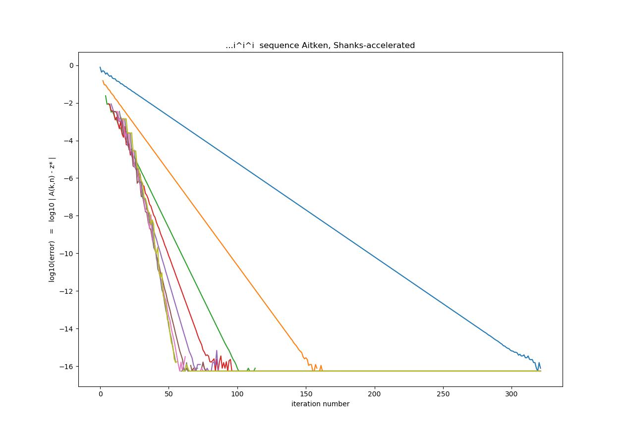
Linear shape of the curves shows that the deviations from the $$z_\infty = 0.43828293672703215 + 0.3605924718713855 \,i\,$$ diminish exponentially as a function of $n$ (location in sequence), as in $$d_n = |z_n-z_\infty| = 10^{-n/\Delta n},$$ where $\Delta n = $ const. The unaccelerated sequence slashes the error $d$ by a factor of 10 in every $\Delta n = 20$ steps or mappings. Aitken process does than in $\Delta n=10$ steps, and high-order Shanks method (Aitken applied 8 times) in just a few steps ($\Delta n \approx 55/16 = 3.44$) on average. It makes no sense doing more than about 7 Shanks accelerations; as you see, the results start getting noisy and do not improve beyond that number.
The minimum numer of steps needed in the optimally Shanks-accelerated
sequence is ~25 to reach a single precision, and ~55 to reach the double
precision. Compare that to 320 steps for double precision in the original
$z$-sequence, which converges to only 1-3 accurate decimal digits
after 25-55 steps. So the acceleration works very well.
It is interesting to
realize that by doing $i^z$ 34 times, we get unaccelerated series accuracy of
about $0.02 \sim 10^{-2}$, while the information sufficient to get accuracy of
$\sim 10^{-10}$ is hidden in this series, waiting to be extracted by your
(I mean Shanks's) cleverness!
How does the speed of Shanks acceleration compare to other iterative algorithms? If you were doing a bisection search for a zero of a function, you would need 22 function evaluations to fix it to a single, and 50 evaluations to a double precision. Similar efficiency. And bisection is actually considered a pretty efficient general algorithm (unless your function is docile and initial guess good enough, in which case you should use Newton's algorithm that works out 15+ accurate digits in under 5 steps.)
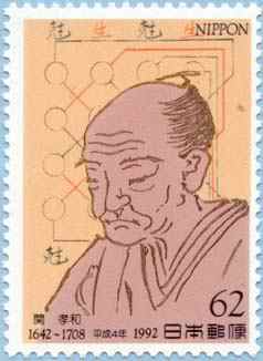 Takakazu Seki, often called Seki Kowa, was a mathematician, samurai, and feudal
officer & master of ceremonies of the Shogun in the city of Koshu at the time of
the Edo Shogunate (Edo is now Tokyo), which lasted from 1603 to 1863.
This high-ranking samurai (hatamoto) discovered but does not seem to get much
credit for: determinants, Bernoulli numbers, maybe also the Newton-Raphson method
we talked about earlier. In 1681 Seki found an acceleration method for series
of partial sums (by a single transformation of series). The goal was to find
a fast-converging representation of $\pi$. He calculated a respectable total
of 10 digits of $\pi$. It must be said that an Austrian Jesuit astronomer
Christoph Grienberger already in 1630 computed 38 digits of $\pi$ using formulae
of Willebrod Snellius of the Snell's law fame, after Ludolf van Ceulen (Ludof
of Cologne, 1539-1610), who started calling number pi $\pi$, computed it to
35 decimals. But these were typically just employing more and more sides in a
polygon inscribed/overscribed on circle --idea due to Archimedes-- or some
linear interpolation of trigonometric series, which is a weaker variant of
acceleration.
Takakazu Seki, often called Seki Kowa, was a mathematician, samurai, and feudal
officer & master of ceremonies of the Shogun in the city of Koshu at the time of
the Edo Shogunate (Edo is now Tokyo), which lasted from 1603 to 1863.
This high-ranking samurai (hatamoto) discovered but does not seem to get much
credit for: determinants, Bernoulli numbers, maybe also the Newton-Raphson method
we talked about earlier. In 1681 Seki found an acceleration method for series
of partial sums (by a single transformation of series). The goal was to find
a fast-converging representation of $\pi$. He calculated a respectable total
of 10 digits of $\pi$. It must be said that an Austrian Jesuit astronomer
Christoph Grienberger already in 1630 computed 38 digits of $\pi$ using formulae
of Willebrod Snellius of the Snell's law fame, after Ludolf van Ceulen (Ludof
of Cologne, 1539-1610), who started calling number pi $\pi$, computed it to
35 decimals. But these were typically just employing more and more sides in a
polygon inscribed/overscribed on circle --idea due to Archimedes-- or some
linear interpolation of trigonometric series, which is a weaker variant of
acceleration.
 The nonlinear method was re-discovered 200+ years later, in the 20th century,
by New Zealander of Scottish descent, Alexander Aitken.
Like Seki before, Aitken was a warrior
(of ANZAC, part of British expeditionary army in WWI, trying to conquer
Bosphorus from Ottoman Turks in 1916). He wrote a widely read book "Gallipoli
to the Somme" (where he was severely wounded in 1918). Known as a mathematician,
one of the best mental calculators, and a man of phenomenal memory, Aitken
was able to recite 700 or, some say, 1000 digits of $\pi$ (that number again!).
But he also had recurrent depression, remembering in all too vivid detail the
horrors of trench warfare. He worked in U. of Edinburgh, with one stint at "Hut
6" in Blatchley Park during WWII, deciphering ENIGMA (for the Allied forces).
The nonlinear method was re-discovered 200+ years later, in the 20th century,
by New Zealander of Scottish descent, Alexander Aitken.
Like Seki before, Aitken was a warrior
(of ANZAC, part of British expeditionary army in WWI, trying to conquer
Bosphorus from Ottoman Turks in 1916). He wrote a widely read book "Gallipoli
to the Somme" (where he was severely wounded in 1918). Known as a mathematician,
one of the best mental calculators, and a man of phenomenal memory, Aitken
was able to recite 700 or, some say, 1000 digits of $\pi$ (that number again!).
But he also had recurrent depression, remembering in all too vivid detail the
horrors of trench warfare. He worked in U. of Edinburgh, with one stint at "Hut
6" in Blatchley Park during WWII, deciphering ENIGMA (for the Allied forces).
 The 3rd person involved, R. J. Schmidt, in 1941 derived Shank's (see below)
later results in Philosophical Transactions. But the interweb doesn't seem to
know about him/her, so the connection to $\pi$ and to a military service is
speculative, if not impossible.
The 3rd person involved, R. J. Schmidt, in 1941 derived Shank's (see below)
later results in Philosophical Transactions. But the interweb doesn't seem to
know about him/her, so the connection to $\pi$ and to a military service is
speculative, if not impossible.
 Last but not least came a re-discovery of the nonlinear series acceleration,
this time in a repeated form, by Daniel Shanks, an American physicist (BSc),
mathematician (PhD in math obtained w/o taking any graduate math courses), and
numericist. His most cited paper is his Phd thesis published as "Non-linear
Transformations of Divergent and Slowly Convergent Sequences" (J. Math. &
Phys., 1955), if you want to read it. Quite fitting for our story, Shanks:
(i) in 1961, using the first transistor-based IBM 7090 computer, computed
$10^5$ digits of $\pi$; (ii) both prior and subsequent to his transformation
from physicist to mathematician, he worked at military proving grounds at
Aberdeen and the Naval Ordnance Laboratory, calculating ballistics and
writing his PhD thesis (though later he worked at National Institute of
Standards, and U. of Maryland.)
Last but not least came a re-discovery of the nonlinear series acceleration,
this time in a repeated form, by Daniel Shanks, an American physicist (BSc),
mathematician (PhD in math obtained w/o taking any graduate math courses), and
numericist. His most cited paper is his Phd thesis published as "Non-linear
Transformations of Divergent and Slowly Convergent Sequences" (J. Math. &
Phys., 1955), if you want to read it. Quite fitting for our story, Shanks:
(i) in 1961, using the first transistor-based IBM 7090 computer, computed
$10^5$ digits of $\pi$; (ii) both prior and subsequent to his transformation
from physicist to mathematician, he worked at military proving grounds at
Aberdeen and the Naval Ordnance Laboratory, calculating ballistics and
writing his PhD thesis (though later he worked at National Institute of
Standards, and U. of Maryland.)