


You may use and modify the codes below. As a minimum, analyze them line by line and run them! Knowledge of structures and methods used in these codes is a course requirement of PHYD57. You must have a basic, passive knowledge of (i.e., ability to understand) both C and Fortran. You will actively program your assignments in one of those languages, as you prefer, unless explicitly instructed to use Python.

Example of speed gain in NumPy vs. pure Python
http://planets.utsc.utoronto.ca/~pawel/progD57/simple_vectors-03.py
All 3 methods
compared. The 3rd method, allocating and filling 1D array with uniformly spaced
floats from a given one to another given number works OK;
np.linspace(a,b,N) program is much faster than the ones containing
Py loops. Actually several dozen times faster.
http://planets.utsc.utoronto.ca/~pawel/progD57/laplacian-5t.py Image processing program. Uses heat/diffusion Laplace operator stencil to thoroughly smear out an image, then subtract it as background from the original image. The method of unsharp masking enhances the image details, removes some overexposure, and any overall gradient or large scale, smooth pattern.
The important part here is the speed of the code. Timing shows that on average, the image (644 x 680 pixels in size) takes 0.00112 s to process once. The equivalent time for 1M pixel image (1024 x 1024) is about 0.00370 s, that is it's done 270 times per second. This is a highly optimized python code (NumPy arrays and their rolling/shifting is used).
By changing the flag to
mode='loop'
you can see that the 1M pixel processing time by Python loops is t = 0.155 s
(done 6.45 times/s). This is 42 times slower! It is likely that Numpy speed is
near maximum achievable, a good example of the power of vectorization (array
operations).
Below we show some advanced coding in Fortran aimed at speeding up the
Python code (though not dramatic speedup will be obtained - NumPy works
great on the Laplacian blurring problem).
http://planets.utsc.utoronto.ca/~pawel/progD57/cudafor-laplace3-dp.f95
This program is written in F95, as its extension .f95 shows.
It uses several different methods to scan a square array (image 1K x 1K),
and apply smearing passes to the image (q=0.2 means nearly max rate of smearing).
CUDA = execution on Nvidia GPU (gtx 1080ti card). Results show that F95 compiler
which knows how to use GPU (Portland Group Fortran 95 compiler) can
compute one Laplace sweep on 1M pixel images (double precision values)
about 9 times faster than Numpy, at a rate of 2.5-3 billion pixels per second,
or 2.5-3 Gpixel/s.
http://planets.utsc.utoronto.ca/~pawel/progD57/cudafor-laplace3-sp.f95
Single precision CUDA isn't (much or not at all) faster than double
precision, and neither is super fast - maybe the problem we solve is too small,
or inefficiently coded in CUDA, e.g. making the time to start all the kernels
significant.
And here are the programs running on host (CPU), which were compiled with two different fortran compilers. They compare the performance of a variety acceleration techniques.
http://planets.utsc.utoronto.ca/~pawel/progD57/ifor-laplace3-dp.f90
is a version compiled by ifort (Intel compiler), and
http://planets.utsc.utoronto.ca/~pawel/progD57/pgf-laplace3-dp.f95
is a version compiled by pgf95 (PGI or Portland Group Fortran compiler).
The programs are identical. The only difference is comments insode on how to
compile them, and quoted results at the end in ifort version. We can spot some
mild differences between the two compiler, however the much more important
difference is timing of different algorithms contained in separate subroutines.
We will discuss those results in class to show you the fundamental reason for the insufficiency of knowing only Python. We will return to these programs and try to rewrite them in C/C++, as we learn Linux, Fortran and C(++). This order is due to the fact that we will use compilers working under Linux operating system (but you should install a Windows/Mac versions on your laptop if you find one), and that Fortran is easier to learn, so it should be learned before C++.
x,y,z,r = 120 125 150 316 cents, P = 711
Next, if price are in cents (to avoid roundoff error in float calculations)
then, for instance, prices like 3 times 1.00 dollar and one time 7.11,
multiply to give 711*100**3 = 711 millions (int).
There is a way to use prime factor decomposition of the product 711000000 =
79 * 3*3 * (2*5)**6, to restrict search to only such integers that contain
factors of 2, 3, 5, and also for one number only, let's call it x, factor 79.
In fact, only 6 possibilies can be shown possible for x: 79, 79*2, 79*3, 79*4,
79*5 and 79*6. Numbers y, z have a combined 105 possible pair values, number r
follows uniquely from x,y,z. So we only check less than 6*105 possibilities.
With right ordering, we actually only calculate 4k to 5k possibilies, which
takes only about a millisecond in fortran.
http://planets.utsc.utoronto.ca/~pawel/progD57/711.py This is the Python code.
http://planets.utsc.utoronto.ca/~pawel/progD57/711.f95 This is the F90 code.
Finally there is a version of the brute force search through a part of cube of
possibile (x,y,z) triplets [the well ordered triplets], which treats not only
7.11 but all numbers from 3.00 to 20.20, as a possible sum and product of four
numbers with two decimal digits after the point. The code is in fortran95.
http://planets.utsc.utoronto.ca/~pawel/progD57/711s-brute.f95 This is the F90 code.
Random sequences that converge when the length of element is used to create a jump to the next element are called Dynkin-Kruskal sequences, after Eugene Dynkin (1924-2014), a Russian-American mathematician, who mentioned them in his work, and American mathematician Martin David Kruskal (1925-2006). The nature of these Kruskal sequences is that they converge exponentially fast, and for N=52 there is already more than 90% chance that the two randomly started sequences converge at the end of the deck, that is the magician and the spectator independently arrive at the same last key card. I saw the trick demonstrated by 50% of Islandic astrophysicists (1 of 2, he said) at one conference, but didn't know that these convergent, linked list-like, series are so common. Almost any books can be used to show that. Skip a number of words equal to the number of letters in a key word. By the end of the third line you normally converge to the same sequence forever after, no matter which word in the top line you start with. Try it! I think almost any book will be good, with a possible exception of a book in German (very long compound words :-).
https://arxiv.org/pdf/math/0110143.pdf is the math paper that explains why the sequences converge.


We programmed a simple loop over a 2-d array in fortran: http://planets.utsc.utoronto.ca/~pawel/progD57/simpler-nb-0.f90. This code does not use any explicit parallelization. Array is declared in the program, not in a separate module, which makes the compiler allocate the array on the stack, not on heap (two different data structures in RAM; google "difference stack heap fortran"). Therefore it is quite possible to get a segfault (segmentation fault) while running the executable, because of limited stack size. To fix that problem, in tcsh shell on art-2 we say something like: % limit stacksize 4000m, while in bash we would use ulimit command (for proper options syntax please see man pages or google it).
The above code is poorly instrumented and we can get only a rough idea of the
speed from running it with time command like so: % time simpler-nb-0.x
(if we have named executable file simpler-nb-0.x). It is better to use
the omp timer omp_get_wtime(), an intrinsic function that returns a double
precision (8B!) result with time in seconds. See code
http://planets.utsc.utoronto.ca/~pawel/progD57/simpler-nb-1.f90.
Data are still on the stack, but the code spits out more information. It interpretes the apparent number of loop passage times estimated FLOP count per passage in two ways: either as FLOPs number or as a result of bandwidth limitation:
$ time simpler-nb-1.x
  done in    36.7159843444824      ms
  throughput   32.68332      GFLOPs << theor. limit
  if bandwidth limited:   130.7333      GB/s
0.101u 0.056s 0:00.16 93.7%	0+0k 0+0io 0pf+0w
art-1[397]:~/avx$
This example shows that this version of the code is certainly not computationally limited, but likely bandwidth-limited, because computations on CPU could go 1 order of magnitude faster. However, look at these 3 different optimization levels while compiling the code, and the numers pronted by the program:
art-1[397]:~/avx$ ifort -O0 -openmp simpler-nb-1.f90 -o simpler-nb-1.x
simpler-nb-1.x
  done in    1158.52308273315      ms
  throughput   1.035802      GFLOPs << theor. limit
  if bandwidth limited:   4.143206      GB/s

art-1[401]:~/avx$ ifort -O1 -openmp simpler-nb-1.f90 -o simpler-nb-1.x
art-1[402]:~/avx$ time simpler-nb-1.x
  done in    356.431007385254      ms
  throughput   3.366711      GFLOPs << theor. limit
  if bandwidth limited:   13.46684      GB/s
0.401u 0.068s 0:00.47 97.8%	0+0k 0+0io 0pf+0w

art-1[403]:~/avx$ ifort -O2 -openmp simpler-nb-1.f90 -o simpler-nb-1.x
art-1[404]:~/avx$ time simpler-nb-1.x
  done in    36.4382266998291      ms
  throughput   32.93245      GFLOPs << theor. limit
  if bandwidth limited:   131.7298      GB/s
0.103u 0.052s 0:00.15 100.0%	0+0k 0+0io 0pf+0w

art-1[405]:~/avx$ ifort -O3 -openmp simpler-nb-1.f90 -o simpler-nb-1.x
art-1[406]:~/avx$ time simpler-nb-1.x
  done in    36.4911556243896      ms
  throughput   32.88468      GFLOPs << theor. limit
  if bandwidth limited:   131.5387      GB/s
0.096u 0.059s 0:00.15 93.3%	0+0k 0+0io 0pf+0w
art-1[407]:~/avx$
Yes, ~150 GB/s is the absolute limit for the RAM bandwidth, actually I think a fantastic result owing partially to an effective use of its cache by CPU. Level -O0 means no optimization, and that's bad for speed, but the standard level -O2 is good. -O3 doesn't give more speedup.


Here is the calling C program for our library:
http://planets.utsc.utoronto.ca/~pawel/progD57/use_libc.c.
Study how these programs are compiled, try them yourself, modify them to your needs (also all the others below). Compilation flag I used awre mentioned in their headers. In particular, option -lfun links the library libfun.so with the program use_libc.c ["lib" is an implied beginning of the .so library].
Now let's compile a library (first, a simplified version w/o
OpanMP part and big array) for use with Python:
http://planets.utsc.utoronto.ca/~pawel/progD57/fun_lib0.c
Here is the calling Python program for library fun_lib0.so:
http://planets.utsc.utoronto.ca/~pawel/progD57/callingC-0-py2.py.
It is, as the name indicates, a Python2 version, since only that version is
fully installed on art-2, where I want you to try compiling and running
programs yourself in user phyd57's sub-directory progD57.
As you see, there are certain tricks that need to be known or googled up, about calling C or other libraries from Python, since it's not trivial. But you do have this template now, so explore and modify it to your needs.
Finally, let's call the full version of the library with OMP.
http://planets.utsc.utoronto.ca/~pawel/progD57/fun_lib.c
Here is the calling Python program for fun_lib.so:
http://planets.utsc.utoronto.ca/~pawel/progD57/callingC-from-py2.py.
We see that the estimates of speed are virtually the same for C calling C library, and Python calling the same library. That's good, it means that the C/Python inteface does not steal any performance, in this example.
Please go back to the links (Lectures 2 and 3) to programs efficiently implementing the cross-shaped stencil of Laplace operator - now you are going to be able to understand the details, such as OpenMP parallelization!
First, a simple CPU version http://planets.utsc.utoronto.ca/~pawel/progD57/tetraDc.f90
And this is the CPU version with changes, can be compiled either with GNU,
Intel or PGI fortran compilers (I believe Intel produces fastest code):
http://planets.utsc.utoronto.ca/~pawel/progD57/tetraDc-3.f90
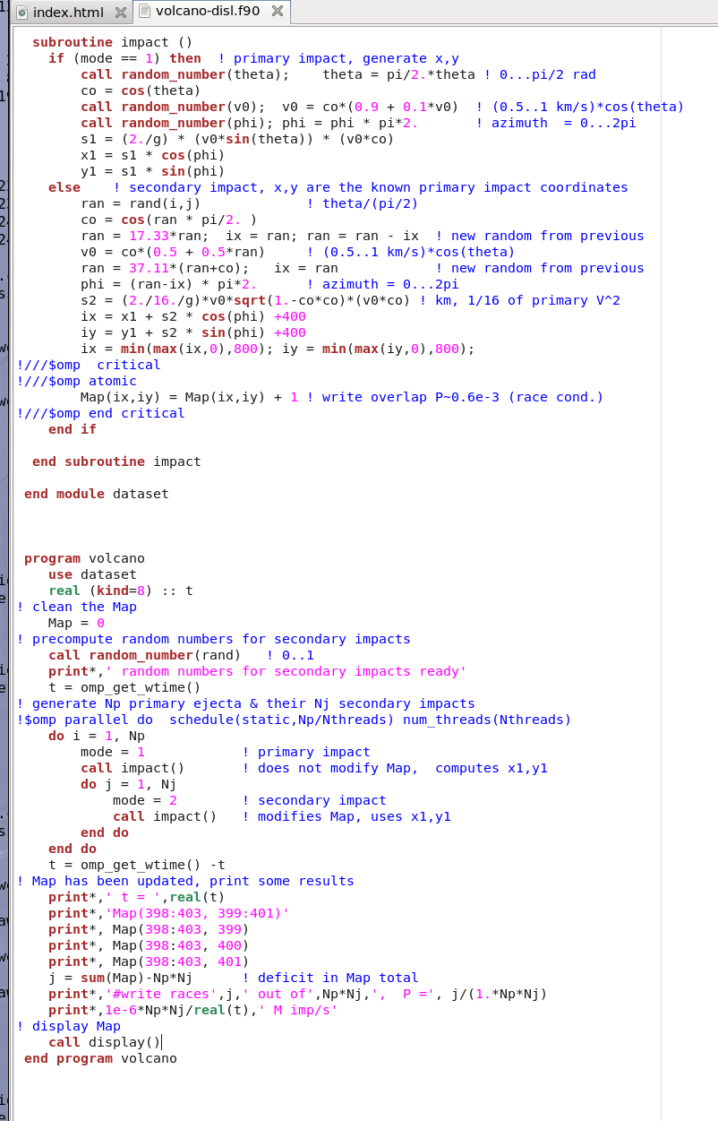
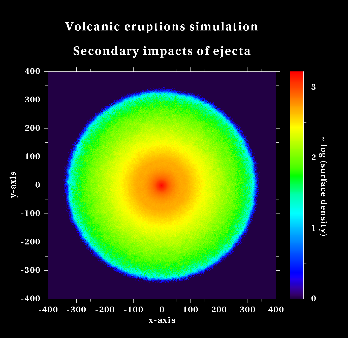
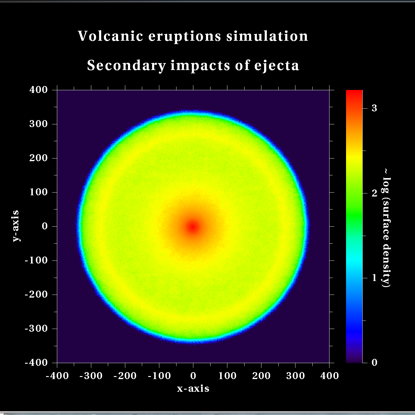
Midterm problem 1 implemented in Fortran, in program volcano-disl.f90 .
See the program below, compile, run.
http://planets.utsc.utoronto.ca/~pawel/progD57/volcano-disl.f90
The crucial computations are done like this (click the nicely colored view):
There is opportunity for you to explore several issues by playing with the program
and running it in art-2's phyd57 account, dislin subdirectory, where it resides:
• How does the compiler (Intel ifort vs. PGI pgf90) affect performance.
PGI produces much slower code, processing ~50 instead ~140 mega-ejecta per sec.
• OpenMP scheduling options, play with it - no big differences.
• Change Nthreads from 1 to 24, see that 12 is optimum
• Insert $omp atomic, $omp critical, around the Map(ix,iy)=Map(ix,iy)+1
update, watch speed drop a few times to 30 times, correspondingly.
That's the price to pay for no contentions while updating Map pixels.
See the statistics printed by the program. We discussed thios in tutorial 6,
and it turned out to be true: probability of simultaneous writing to a
pixel location (race condition resulting in one or both updates being dropped)
is only P < 0.001.
• different ranges of V
v0 = co*(0.5 + 0.5*v0) -> v0 = co*(0.95 + 0.1*v0) (see the ring?)
• Notice that I generate one random number per impact only. Pseudorandom
float contains quite a few random digits, therefore one can generate three (like
here) or even more slightly more coarse-grained pseudorandom floats from it.
Even though I didn't see much speedup from this trick, it saves substantial amount
of memory.
• Read and learn the usage of DISLIN from the the preceding, as well as
these two codes (compilation instructions inside):
ex11_1.c
and
ex11_1.f90
CUDA C blog by Mark Harris, NVIDIA <== recomended
CUDA C presentation - different modes of usage, by Cyril Zeller, NVIDIA
CUDA C Programming Guide. Detailed. Definitive (By Nvidia!). Read first 30 pages.
CUFFT library description - useful when you need FFT. Some learning curve, but once you get it to work, the world of DSP is yours. Has examples of all fft's (complex to complex, real to complex etc.).
Paper comparing CUDA in Fortran and C with CPU performance, as a function of job size.
Dr. Dobbs blog CUDA, Supercomputing for the Masses. Links to all 12 pieces. A bit old but informative.
Cuda programming model - Refresher.
SAXPY
In the phyd57/progD57 account on art-2 you can find these three simple tests
of the basic saxpy (meanig: single-precision float a*x+y) i.e. the
basic linear algebra operation.
http://planets.utsc.utoronto.ca/~pawel/progD57/simple_saxpy_cuda-.cu (sometimes we give extension .cu to CUDA codes written for nvcc compilation, but here it's a version for CPU, never mind!)
http://planets.utsc.utoronto.ca/~pawel/progD57/simple_saxpy_cuda.cu. This
one does the honest CUDA kernels.
http://planets.utsc.utoronto.ca/~pawel/progD57/cuda-perf.f95. F95 version with more diagnostics, showing bandwidth, compute performance, and a way to
call shell commands from within the program.
Diffusion stencil computation
This is a GPU version of the 5-pt stencil Laplacian code you have seen before;
written in part using CUDA Fortran; to be compiled with the PGI compiler pgf95.
This version is dp (double precision floats, 8B), there is also an sp version (single
precision float, 4B) with a similar name on art-2.
https://planets.utsc.utoronto.ca/~pawel/progD57/cudafor-laplace3-dp.f95.
Tetrahedra on graphics gear
This is a GPU version of the code you may have seen before if you were interested in tetrahedra; written in part using CUDA Fortran; to be compiled with the PGI compiler pgf95. https://planets.utsc.utoronto.ca/~pawel/progD57/tetraDg-3.f95.
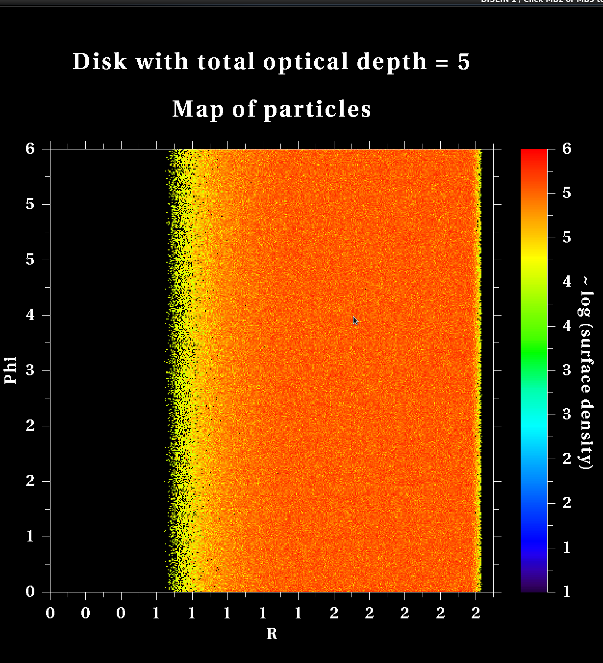
tau-dis-cpu.f90 although it works, has some problems. Find and remove them


Partial summation of infinite series over 1,2,3,...,k terms has the form:
exp(x) = ex = 1 + x/1! + x2/2! + x3/3! +
+ ... + xk/k! + ...
Factorial function k! is defined as k! = 1*2*3....*(n-1)*n As you see, we do not need to start this multiplication from scratch doing repeated loops over k=1,2,3,.. . Rather, since n! = n (n-1)!, we simply start from the first (lowest) value of (n-1)! and repeatedly update the factorial variable in every loop passage. See the code.
We keep the always improving partial sum of the series terms (functions) and call it y. We plot y vs. x for every k. We stop at k~20,
http://planets.utsc.utoronto.ca/~pawel/progD57/plot_cos_approx-1.py Cosine function series approximation.
The figure constructed with MatPlotlib shows that the larger the absolute value of
the argument x, the more terms are needed for a good approximation of
the function exp(x), both for positive and negative x.
Remark: use the zoom button on the plotting widget that your Python installation
provides. This way you can disentangle particularly dense parts of the figure!
Another example of the same type of simple overplotted lines with automatic
coloring by PyPlot.
http://planets.utsc.utoronto.ca/~pawel/progD57/plot_cos_approx-1.py does the same
as above with the trigonometric function cos(x).
Taylor (MaclLaurin) series of it is given by
cos(x) = 1 - x2*1/(2*1)! + x2*2/(2*2)! + x2*3/(2*3)! +
+ ... + x2k/(2k)! + ...
epi-4.py, ;nbsp& epi-5.py, epi-6.py, epi-7.py, epi-8.py, epi-8B.py
http://planets.utsc.utoronto.ca/~pawel/progD57/simple_IO.py shows how to read and write to/from ASCII files, comma or space-separated values.
http://planets.utsc.utoronto.ca/~pawel/progD57/simple_stat.py shows how to compute (in 3 different ways) simple statistics, like the average values and two kinds of sigmas (st. dev. of the data, std dev of the mean), for data read from files.
http://planets.utsc.utoronto.ca/~pawel/progD57/kepl-GJ-3512b.py
Planetary system
around a small M5 dwarf star not far from Earth (10 pc) was discovered and
announced in late 2019. Media say it's a big discovery challenging
the existing planet formation theories. Not necessarily.
Planets is on eccentric orbit, and the program produces not only the visualization of planet's uneven, eccentric motion but also the correction to mean flux received on the planet because of e=0.4356. It even computes the temperature of the planet.
http://planets.utsc.utoronto.ca/~pawel/progD57/expfract-s1.py Exponential (Artymowicz) fractal calculator
http://planets.utsc.utoronto.ca/~pawel/progD57/expfract-p1.py Exponential (Artymowicz) fractal calculator, diffrent color map & region
http://planets.utsc.utoronto.ca/~pawel/progD57/histo3.py Generate a bunch of random numbers and show their histogram. Compares uniform and normal distributions.
http://planets.utsc.utoronto.ca/~pawel/progD57/simple_mtc_pi.py Calculation of Pi by Monte Carlo. A classic of MtCarlo demonstrations. Simple version.
http://planets.utsc.utoronto.ca/~pawel/progD57/simple_mtc+int_pi.py Calculation of Pi by Monte Carlo. This version compares the Monte Carlo accuracy with a regular integration on a uniform mesh of N points, the same number as MtC particles (so, similar computational effort). We begin to see the problem with MtC: 1/sqrt(N) signifies the slow convergence to zero value of error.
http://planets.utsc.utoronto.ca/~pawel/progD57/Radioactive.py Calculation of decay histories of radioactive isotope U-235 by Monte Carlo simulations. Compares different realizations of the experiment in one plot.
http://planets.utsc.utoronto.ca/~pawel/progD57/dusty-box-1.py
Dusty box, or rather a dusty duct, is simulated to see how we can solve a basic
radiation transfer problem by randomly placing absorbers in the field of view.
It turns out, we can reproduce very exactly the analytical result I = I0
exp(-τ).

 On the left is a layer of clouds with τ>>1, which we analysed in Lecture 5.
Bay of San Fancisco, 21 July 2019. And to the right, I photographed
the optically thinner cloud
(τ ~ 3.6?) not of water droplets but smoke and ash particles from
forest/grass fires near Meteor Crater, AZ, 19 July 2019.
On the left is a layer of clouds with τ>>1, which we analysed in Lecture 5.
Bay of San Fancisco, 21 July 2019. And to the right, I photographed
the optically thinner cloud
(τ ~ 3.6?) not of water droplets but smoke and ash particles from
forest/grass fires near Meteor Crater, AZ, 19 July 2019.
http://planets.utsc.utoronto.ca/~pawel/progD57/rnd-walk-gamble-0.py Multiple 1D (i.e., 1-dimensional) random walks on one plot. This simulates diffusion in physics, paths of photons in the sun, or some extremely large Galton board, flight of an arrow through a turbulent air, how perfume spreads in still air, how heat speards through solids, and/or a number of other things. No restrictions on the range of random walk in this version.
http://planets.utsc.utoronto.ca/~pawel/progD57/rnd-walk-gambles.py provides a modified version of 1D RND Walk, with absorbing boundary at X=0 (a.k.a. Gambler's Ruin Problem).
http://planets.utsc.utoronto.ca/~pawel/progD57/err_d1f-3.py Thorough error analysis, both roundoff and truncation error, analytical and numerical, of two stencils for first order derivative. Demonstrates the advantages of high order stencils.
http://planets.utsc.utoronto.ca/~pawel/progD57/simple_bisec.py Bisection method of root search of a 1-D real function. Illustrates the generally robust performance and the possibility of missing some zeros.
http://planets.utsc.utoronto.ca/~pawel/progD57/simple_secant.py Secant method of zero finding of a 1-D real function. There was a bug in the program, now converges as fast as it should, and in fact impressively fast, 'superlinearly', almost like Newton's scheme, in less than 8 steps as a rule.
http://planets.utsc.utoronto.ca/~pawel/progD57/simple_newton.py Newton's method of zero finding of a 1-D real function. Illustrates the relatively fast convergence in the case of 3rd order polynomial function. When it works, it works really great. When it fails, it fails like no other algorithm. Can you say when?
http://planets.utsc.utoronto.ca/~pawel/progD57/compare_sqrt-2.py Comparison of all three methods of finding zero efficiently, one of them (Newton's) is run in two variants: with numerical and analytical derivative calculation. One can see the huge advantage of those methods which converge quadratically or at least faster than linearl, meaning that the next error is asymtotically proportional the a power of the previous error larger than 1., sometimes 2.
http://planets.utsc.utoronto.ca/~pawel/progD57/oxford-IO-2.py
and a variant
http://planets.utsc.utoronto.ca/~pawel/progD57/oxford-IO-3.py
Archival data from Oxford, UK, weather analysis 1929-2010.
Monthly data on # of sunny hours per month, which is used in this exercise,
is in this file:
http://planets.utsc.utoronto.ca/~pawel/progD57/oxford_sunny.dat
http://planets.utsc.utoronto.ca/~pawel/progD57/integ-p124-arc.py compares the convergence of several simple 1st to 4th order integration schemes of the function 1/(1+x*x) between x=0 and x=1. Name derives from Arctan(x) which is an analytical integral value. BTW, all of the integration codes have known exact answers, mostly involving number π . These codes therefore calculate that number numerically.
http://planets.utsc.utoronto.ca/~pawel/progD57/integ-p124-exp.py compares the convergence of several simple 1st to 4th order integration schemes of the function exp(-x) between x=0 and x=1.
http://planets.utsc.utoronto.ca/~pawel/progD57/integ-p124-cur.py compares the convergence of several simple 1st to 4th order integration schemes on the problem of the length of the curtain as a line integral using Pythagoras theorem, or an integral of (1+(y')**2)**0.5 where y is the curtain's shape and y'=dy/dx. This turns out an easy problem for numerical integration schemes!
http://planets.utsc.utoronto.ca/~pawel/progD57/integ-p124-Acirc.py compares the convergence of several simple 1st to 4th order integration schemes of the function sqrt(1-x*x) (1/4 of a circle between x=0 and x=1). This function poses a lot of problems for numerical integration schemes, because of its unbound derivatives as x-->1.
http://planets.utsc.utoronto.ca/~pawel/progD57/integ-p124-Lcirc.py compares the convergence of several simple 1st to 4th order integration schemes of the length of curve qrt(1-x*x) (1/4 of a circle between x=0 and x=1). This integration also poses a lot of problems for most numerical integration schemes, because of its unbound derivatives as x-->1.
http://planets.utsc.utoronto.ca/~pawel/progD57/fit-3par.py solves the linear least-squares fit problem. The function has 3 parameters (amplitudes) multiplying a parabola. Data have a moderate amount of noise added. Program restores the parabola, hence denoising the data.
http://planets.utsc.utoronto.ca/~pawel/progD57/fit-4parN.py solves the linear least-squares fit problem. The function has 4 parameters (amplitudes) multiplying a parabola plus a cosine function of known period. Data includes noise. Program successfully restores the hidden truth (line), hence denoising the data.
http://planets.utsc.utoronto.ca/~pawel/progD57/fit-4par-N2.py solves the linear least-squares fit problem. The function has 4 parameters (amplitudes) multiplying a parabola plus a cosine function of known period. Data has a large amount of noise added, making it visually difficult to separate smooth functional dependence from quasi-Gaussian noise. Despite this, program fairly successfully restores the smooth underlying function/denoises the data, although the quality of parameter restoration starts to suffer (esp. curvature a[0] is too low).
http://planets.utsc.utoronto.ca/~pawel/progD57/diff1-throw-6.py
This program fort simulates a throw of ball (or arbitrary test mass) in vacuum.
Notice that the air drag will be studied in Lecture 11. Initial conditions:
(x0,z0) = (0,0) & (vx0,vz0) = (70,20) m/s.
http://planets.utsc.utoronto.ca/~pawel/progD57/diff1-ex3.py
1-D ODE integration; solve dy/dx = f(x,y) = -sin(x)*y,
with boundary cond. y(0)=1, & various integration schemes.
http://planets.utsc.utoronto.ca/~pawel/progD57/diff1-ex3L.py
Same as above but
over a 10 times longer period of time. Despite an initially high precision of
some methods, a drift in solution becomes evident. This is bad news, as it is
enough to just wait until the drift destroys the initial accuracy.
http://planets.utsc.utoronto.ca/~pawel/progD57/phys-pendulum.py
Motion of a physical pendulum (able to go to the top and over the top on a
rigid massles arm, depending on initial conditions.
The script implements a Leapfrog algorithm, but looks deceptively simple like
Euler method. Not only does it not do the half-step with positions, full step
velocities and again half-step with positions, but also does not star in a
special way to separate speeds and positions in time by dt/2... yet it is
accurate (2nd order accurate).
This is the
diffraction-interference pattern from two slits on a screen 1 m away.
Slits are 30 microns wide, spaces 240 microns apart.
http://planets.utsc.utoronto.ca/~pawel/progD57/inteference-1.py
Compare the pattern with the pattern of diffraction on one slit! And click on
the middle illustration above. You'll see the red laser interference fringes
in the actual experiment on the right hand side.
http://planets.utsc.utoronto.ca/~pawel/progD57/pond1.py
This code is deliberately a little buggy and slow. But that's how one would
very naively approach the solution of the 2-D
linear wave equation:
u_tt = c**2 (u_xx + u_yy)
using Python loops (hence slowness!)
http://planets.utsc.utoronto.ca/~pawel/progD57/pond3.py
shows a wave pattern from an initial disturbance of a pond near the corner.
Algorithm uses only Z arrays (different copies for new, current, and
previous time step of array Z.
http://planets.utsc.utoronto.ca/~pawel/progD57/pond4.py
shows a wave pattern from a localized initial disturbance far from the boundary.
This algorithm is only slightly different, introduces explicitly
V array which is first time derivative of array Z (times dt).
Run at about the same speed(?) as pond3.py.
http://planets.utsc.utoronto.ca/~pawel/progD57/pond4-1obj.py
shows that one can force not only boundary conditions on the walls, but also
in the middle, creating a region impermeable for waves.
http://planets.utsc.utoronto.ca/~pawel/progD57/pond4-2slits3.py
This is the famous double slit experiment simulated on water surface or as
soundwaves (no quantum mechanics here, though QM experiment is strictly
analogous and creates diffraction-interference patterns for the same reason.