Lectures, Tutorials, Office hours, UofT Code of Conduct

Tutorials are NOT meant for the explanation of Lectures - they deal with implementation of methods and calculations sometimes, but not always discussed in lectures. If you want a good grade, please come to tutorials. There will be short quizzes, those on due dates for assignments will be graded. Together your attendance and work at tutorials is worth 12% of the mark.

Office hours: one, sometimes two hours after lectures, minus lunch break. I am open to discussions about the course, computing and supercomputing, astrophysics, academic career, aeronautics, or the meaning of life, universe and everything, at most times when I'm in my office. Please drop by and if I'm too busy then you can always come later.

The Code of Behaviour on Academic Matters at UofT needs to be followed. If you have not read it, you may unknowingly find yourself in trouble. This document succinctly defines conduct that constitues plagiarism, i.e. misrepresentation of authorship, e.g., cheating that the assigned work is yours and original, while you merely rephrase somebody's code by changing its appearence; it is an equal offence to help somebody plagiarise your own work). The Code mentions how reasonably grounded suspicions must be addressed by your Instructor, Dept. Chair, and so on. Read more here.

Contact

Your TA and expert on Python and computing will be Fergus Horrobin ( horrobin@astro.utoronto.ca ). You'll be meeting him in tutorial sections from 16:00 to 19:00 on Tuesdays.

Books

Our main textbooks are

1. J. Izaac and J. Wang, "Computational Quantum Mechanics", Springer 2018.
2. P. Turner, T. Arildsen, K. Kavanagh, "Applied Scientific Computing with Python", Springer 2018.

Please read chapter on Python in book 1. Selected parts of the second book will be used after midterm: chapters 3, 5, 6, 7.

The first book has a nice, short introduction to Python3, the language we will be learning. Do not despair if you don't know Quantum Mechanics, it is not needed; we skip the whole last part of the book. The second book also uses Python but is much less concerned with programming and more with the numerical methods for scientists.

Additional, non-required books for those who want to know Python well. Either one of these is good:

3. H. Langtangen, "A Primer on Scientific Programming with Python", 5th ed., Springer, 2016
4. S. Linge, H. Langtangen, "Programming for Computations - Python", 1st ed., Springer, 2016

Book 4 is a much shorter, different, version of book 3. Lots of practical, short code snippets, and tips on various modules. BUT books 3 & 4 use Python ver. 2, which has some differences with Python 3 syntax. One can learn about them online, e.g. from the first few section on this page. The differences in input/output and integer division seem quite manageable, and other things are less important; you will program by reference to the official Python 3 pages on python.org (see the links section below). In fact, Linge's book just appeared (in Fall 2019) in new edition with Python3 replacing the occasional version 2 syntax.

Lectures will follow the topics mentioned in textbooks 1 & 2, but not in the particular order or wording. Please pay attention to material taught in lectures, most of what is said in lectures will be reflected in lecture notes and code examples page. Run and analyze sample codes line by line, try to improve and develop them to do more things, change their output. That is how programmers learn programming. Hearing lectures without running and modifying programs is not enough.

Course grading scheme

Lecture notes in PDF

Please follow the links in lectures. Also, study the first two Links (on the list below). Knowledge of basic terms (bit, byte, bandwidth, various prefixes like K=Kilo=1024, M=Mega=1024^2, G=Giga=1024^3, and what powers of 2 and approximately which power of ten) will be required!

Lecture 1       Lecture 2       Lecture 3       Lecture 4
Lecture 5       Lecture 6       Lecture 7       Lecture 8
Lecture 9       Lecture 10     Lecture 11     Lecture 12

Code page

Assignments

Submission format was explained during tutorial. You submit to Quercus jupyter notebooks, which are .ipynb documents, saving whatever you type in a Jupyter notebook, e.g. your Python3 scripts, descriptions and pictures.

Problems set 1 . Update consists of 4 problems. Due date 1 October.
Problems set 2 . Published 27 Sept, Due 8 Oct (Tue).
Problems set 3, due on 8 Nov.
Problems set 4 , due on 28 Nov.

Midterm exam

Text of the midterm with solutions is published here as an aid to preparation for the final. The script that solves the problem section is here

Tutorials

Final exam

Solutions to the exam are here

Results

Links

• http://www.linfo.org/bit.html . Concept and history of bit (b). Please study it, and follow links to other important basic concepts in that short article, which you will be required to understand and define during exams and quizzes, such as: bitrate, bandwidth, data bus, 32- vs. 64-bit systems, ASCII code, pixels, various powers of 10 in computer lingo, and RAM memory. Note that this online encyclopedia is slightly outdated as (from 2004); in 2019 "current" hardware capabilities are a bit higher (pun intended).

• http://www.linfo.org/byte.html . Concept and history of byte (B). Another bunch of important basic terminology. From now on, a telemarketer won't be successful in the push for you to buy his new "300 Gigabyte" internet home service -- you'll explain to him/her the difference between bits and bytes.

• https://wiki.python.org/moin/BeginnersGuide/Programmers Introductions of all sorts to Python language for beginnig coders. (Yes, that's you.)

• https://docs.python.org/3.0/reference is Python Language Reference straight from the horses mouth.

• https://docs.python.org/3.0/reference/index.html offers other docs and resources on Python

• tutorial on MatPlotlib

• https://docs.scipy.org/doc/numpy/index.html. Tutorial and user guide to NumPy

• https://matplotlib.org/3.1.1/tutorials/introductory/pyplot.html. Tutorial on Pyplot (part of Matplotlib based on MATLAB syntax).

• https://en.wikipedia.org/wiki/Marian_Rejewski . Are you interested in ENIGMA and its decoding before and during WWII?
Then you have to dig deeper than the related Hollywood movies, which are at times extremely short on real history (better cf. Max Hastings, "The secret War: Spies, Codes and Guerillas 1939-1945", London, 2015). ENIGMA machines were used by Hitler's military for coded communications between the headquarters and units in the field. ENIGMA decoding, first achieved in Poland by Marian Rejewski's team, may eventually have preserved millions of lives, by saving England from German invasion, tipping the balance in favor of Allies, and shortening the world war.

After the pre-war Polish cryptologic breakthroughs, hardware devices were built there, implementing the decoding algorithms called Bomba (cryptographic bomb; or "bombe" in top-secret U.S. Army reports of the time). https://en.wikipedia.org/wiki/Bomba_(cryptography). Copies of ENIGMA machines were also built. Eventually an even faster hacking of the gradually more complex combinations of wheels inside ENIGMAs became necessary.

This was undertaken by British government using qualitatively the same approach as invented by the secret Polish Cipher Bureau. An electromechanical version of the Polish Bomba was built in Blatchely Park near London by an outstanding pioneer of computational science Alan Turing. He also created some statistical theory to aid this work.
The recent biographical movie on A. Turing and the British Enigma-cracking machinery titled "The imitation game" distorts the history, as his team is incorrectly given the sole credit for breaking ENIGMA code. In fact they were neither the first not the last to come up with essential breakthroughs. For instance, a half-forgotten team of brilliant engineers of the British Post Office headed by Thomas Flowers working around the clock for months constructed the specialized Colossus computer and transferred it to Turing's bureau. That device is shown in the movie, but was neither Turing's invention nor was tasked with deciphering ENIGMA codes! Instead, it dealt with other, non-ENIGMA German codes.

Even more powerful machines were developed during the WWWII by American government (Navy), in order to decipher the changed coding procedure used by German submarines. Such devices were the first computers, though not general-purpose electronic computers we have today. They were mostly electromechanical, that is to say based on relays and automatic switches.

As you see, computing from the beginning was and continues to be very very useful. Unfortunately these days it is often used for spying on... you. You do have a smartphone? Anyway, enjoy the four ENIGMAtic movies nicely broken down for you on this page .

• https://www.top500.org". Supercomputing stats. Explore the site, incl. the most recent list of the fastest supercomps in the world at https://www.top500.org/list/2019/06/.

• https://www.researchgate.net/post/Why_are_physicists_stuck_with_Fortran_and_not_willing_to_move_to_Python_with_NumPy_and_Scipy .
Python vs. Fortran. This nice discussion on Stackexchange (the often informative resource for coders) will likely answer more questions than you have on what are the essential differences between Python and high-level compiled languages - here Fortran (a good example, maybe the best one, of such languages; C/C++ is another).

https://arstechnica.com/science/2014/05/scientific-computings-future-can-any-coding-language-top-a-1950s-behemoth/ proposes: "It certainly seems likely, in light of the above, that Fortran will remain the fastest option for numerical supercomputing for the foreseeable future—at least if 'fast' refers to the raw speed of compiled code. But there are other reasons for Fortran’s staying power."

I prefer Fortran for demanding research and Python and/or another scrpting language IDL for small tasks and everything else. C/C++, in which (Unix and) Linux operating systems are written, is useful too, as it sometimes provides the most direct way to tinker in strange ways with graphics cards (GPUs) to make them do CUDA. [That is an inside joke for people coming from my part of Europe. CUDA is the extension of C/C++ (and Fortran) that directs data transfer to/from CPU and computation on GPU. Appropriately, the word spelled "cuda" means "miracles" in most Slavic languages, and in Hungarian (csodak)]. We will deal with such miracles in course PHYD57 Advanced Computing for Physical Sciences, which you may consider taking. Its premiere comes in Spring 2020.

Notes on special topics

Here we will provide some concise notes on special topics discussed in lectures, which are not found in our textbooks.

This is just an example:

Numerical investigation of chaos in Hills equations

Problem of near-Earth motion of a satellite or Moon, neglecting the mass of the 3rd body (circular restricted 3-body problem), in addition done very locally around a small planet, so that everything except planet's gravity can be linearized.
Mathematical formulation of the problem:
dx/dt = v_x
dy/dt = v_y
dv_x/dt = -3x/r³ +2v_y +3x
dv_y/dt = -3y/r³ -2v_x -v_p/2
where: r² = x² + y².
The parameter v_p is the nondimensional radial speed of a migrating planet, and you may set it to zero, if you want the standard R3B problem. The terms on the r.h.s. of the first eq. are: Earth's gravity, Coriolis force due to frame rotation, tidal force (in x-equation only). We don't see either mass of the planet, G constant, or frame rotation rate (Ω), because the above equations are nondimensionalized (all these constants have been divided away, and for instance x stands for the original x divided by r_L, the Hill sphere or Roche lobe radius).

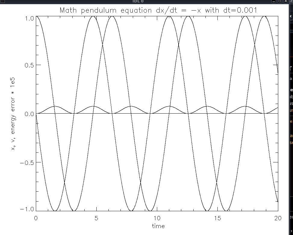
In tutorial we study the integration schemes of 2nd order Euler, and Leapfrog (Verlet) method. I used IDL (Interactive Data Language) scripts that also run under GDL (free IDL), and you are encouraged to rewrite them in Python 3. Both IDL and Python are dynamically typed, interpreted languages, no major differences except that IDL has been established in astrophysics world much earlier.
inte1.pro
inte2.pro
inte2.png (results of inte2.pro)
Later, you can study this program: hill.pro
Examples of results are here:

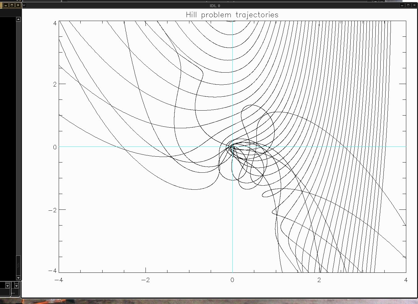
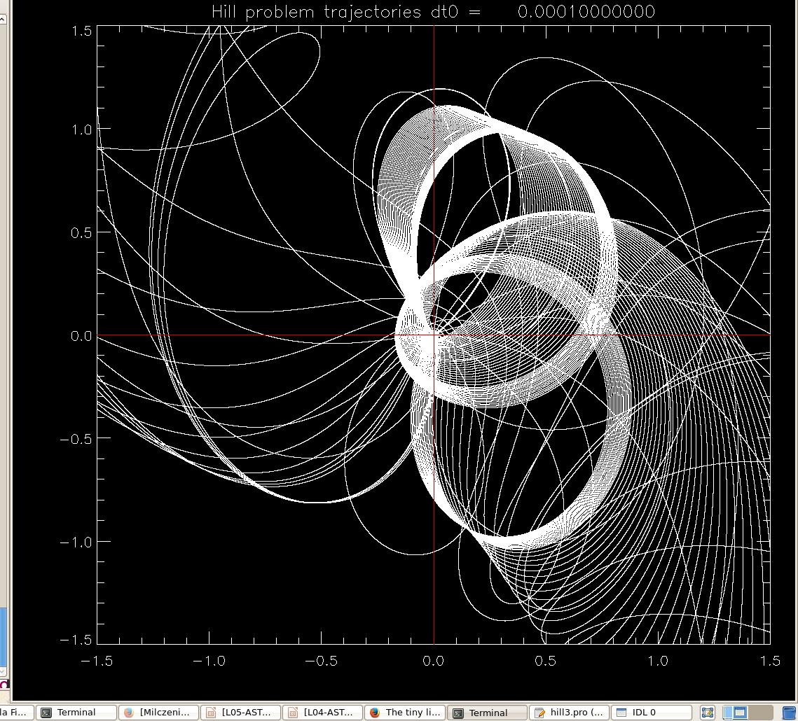
Program hill3.pro was used to produce these picture. It solves Hill's problem for a range of starting positions outside the orbit of the planet (positive radial coordinate x). Vertical motions are neglected, but you can add the z-equation to the system, the only z-force is from the planet, so it will look quite similar to the x and y forces.
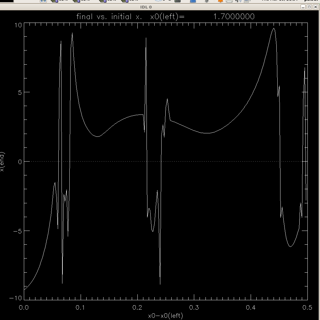
We start by identifying larger scale features x-y view of orbits (units are Hill sphere radii) , and the corresponding graph of
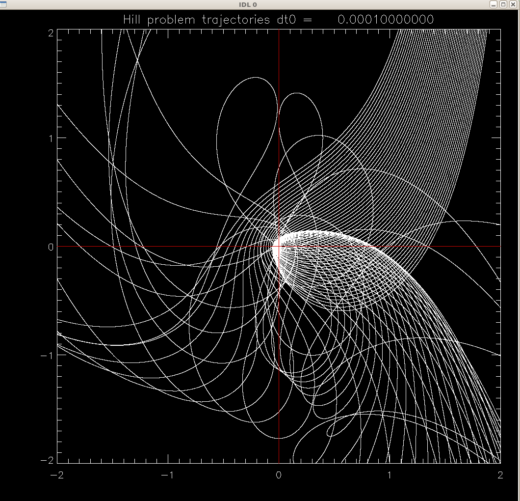
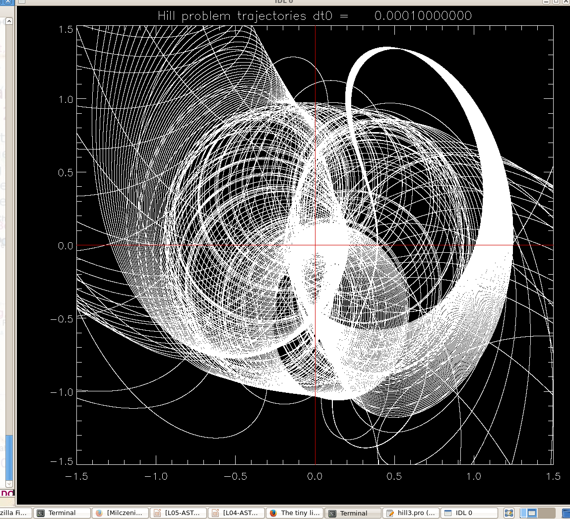
function x(x0) . Not clear if it's chaos. There are ways to estimate the so-called Lyapunov exponents, to answer such a question. Or one can start zooming in ...

A dog, a duck, and the mystery of an invisible magnet

SOLUTION
There are different kinds of solutions. Some of you would prefer to find a numerical solution first, while others the analytical solution first. Both are good choices for the first stab at the problem, as long as you attempt the other kind of method as well. As a matter of fact, if you start with numerical solution then you're immediately faced with the problem of what equation to ask the computer to solve. Let's talk about that first, then. I will use a compact kind of notation, using complex numbers in place of vectors, although at the cost of writing twice as many equations one can work directly with (x,y) or with (r,φ) coordinates of the dog in the program. Complex numbers just look.. less complex in a program. You may think of them as vectors, which they are. Let the position of the dog be r = x+iy, and D be another complex number giving duck's position.

The dog goes straight for the duck, so along the vector D-r, at speed s, i.e.
dr/dt = s (D-r)/|D-r|
where the ducks position is known to uniformly move in a unit circle:
D(t) = exp(it).
That's not the end, since both animals are moving in some circular or quasi-spiral way. Rather than talk about position r(t), we'd better switch to vector R,
R = exp(-it) (D-r)
which is an instantaneous vector from the dog to its moving target, in a reference frame that rotates at uniform unit speed with the duck. In such a rotating frame, the duck is always at (0,0) position and R won't run wildly in quasi-circles, obscuring the plot. The required frame rotation is accomplished by turning any vector to the right by t radians, which is easily done in complex plane with multiplication by exp(-it).
We work out, by differentiation of the definition, the derivative of R to be
dR/dt = -i exp(-it) (D-r) + exp(-it) [dD/dt - dr/dt].
Taking into account that dD/dt = i exp(it), and that dr/dt=sR/|R|, we obtain our evolution equation for a 2d dynamical system in the complex form

dR/dt = s R/|R| + i(1-R)

The numerial solutions in GDL for R(t), t=0...500, were obtained with this second-order integrator (dt = 0.004 was sufficient for accuracy), for a series of 20 uniform spaced values from 0 to 1 (s = 0.05, 0.1, 0.15, ...).

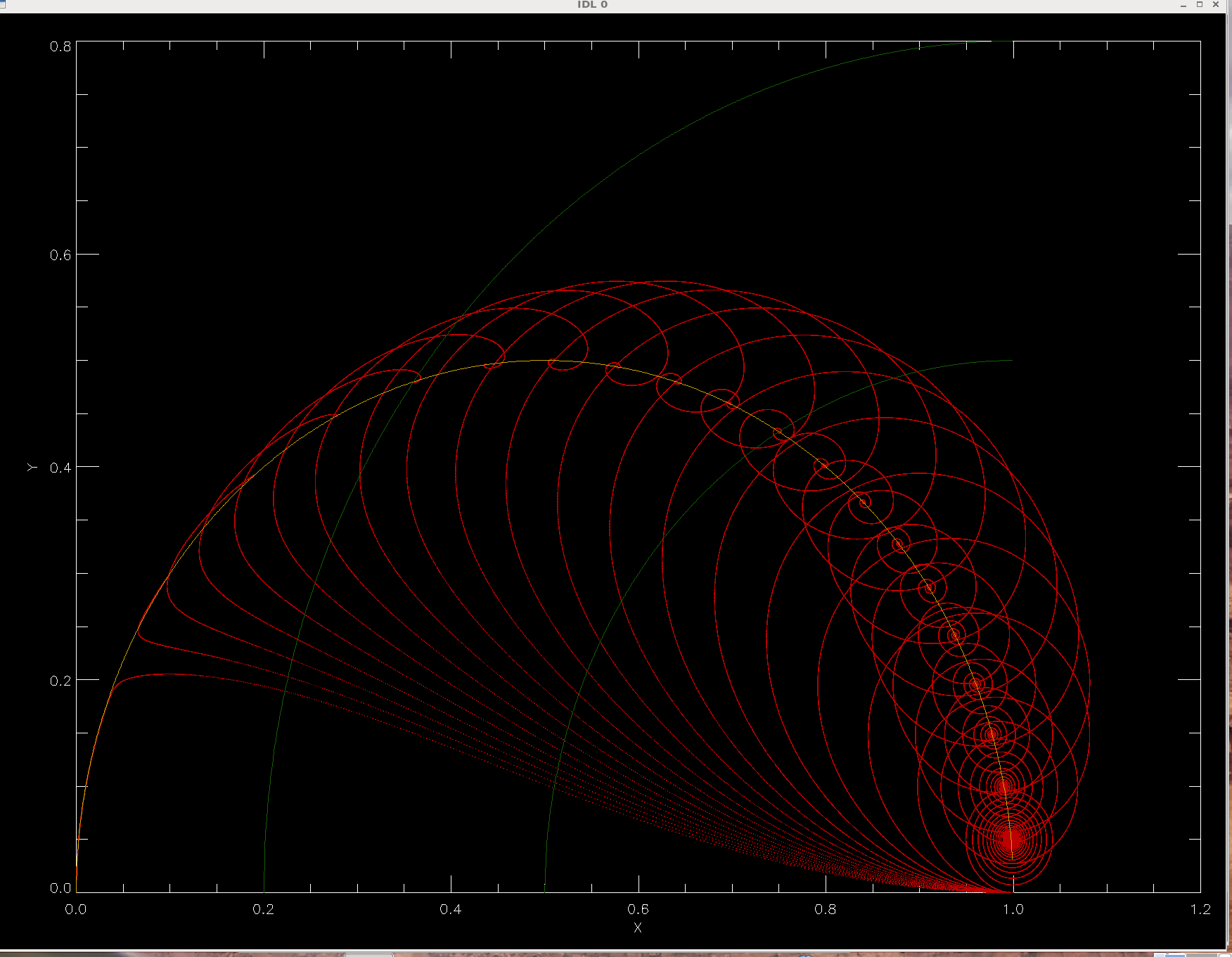
The higher the dog's speed s, the closer to the duck it eventually gets. For s=1, it reaches the duck in infinite time (and for s>1 in finite time). In every case, there is a fixed point to which the solution tends over the time of integration. Two green lines in the plot are circles drawn around the center of the pond (1,0), and have radii |R-1|=0.5 and 0.8 of the pond radius, for illustration of an important fact: the position of a (moving) dog with respect to (moving) duck tends to the radius equal s, as long as s is not larger than 1. You can see that two of the plotted trajectories (for s=0.5 and s=0.8) end at radius s.

We didn't have to do numerical solutions to find this fact, or even the precise asymptotic positions. Fixed positions can be found analytically from the evolution equations, as usual. Zeroing the r.h.s. we obtain R* (we'll skip the * for simplicity, to avoid confusion with dot product or multiplication):
i(R-1) = s R/|R|.
Taking absolute value of this equation, we get |R-1| = s, precisely the point we have noticed empirically; R-1 is the final position of the dog in the rotating frame (dog enters a limit cycle that is a circle of radius s in non-rotating plane). Now we've proven it. Notice that we can also prove it ad absurdum: If |R-1| were not equal to s, the dog in its fixed position relative to the duck would travel at a linear speed differing from s (their angular speeds in fixed configuration being the same, the dog's linear speed is equal to its radius |R-1|, but that number would be different from s). This is a contradiction.
Furthermore, (R-1) as a vector is perpendicular to R, because the complex numbers representing them differ by a factor i/s, which represents re-scaling by (1/s) and rotation by 90 degrees.

What is the locus of points such that vectors drawn from (0,0) and (1,0) to those points are at right angle? It's a circle whose diameter joins the two points, according to an ancient Greek geometry theorem. We can prove it by writing the usual equation for the sought-after curve in terms of coordinates x and y. We have R =(x,y), so the dot product of the two vectors R-1 and R must vanish: (x-1,y)*(x,y) = 0. This can be written as either x(x-1) +y² = 0 or more familiar form of the equation of circle (x - 1/2)² + y^2 = (1/2)². This is such a valuable result that we color half of this circle gold in our plots. So the fixed points are at intersection of two circles with radii 0.5 and s, trailing the motion of the duck by an angle θ = arccos(s). The family of solutions makes a beautiful shell:

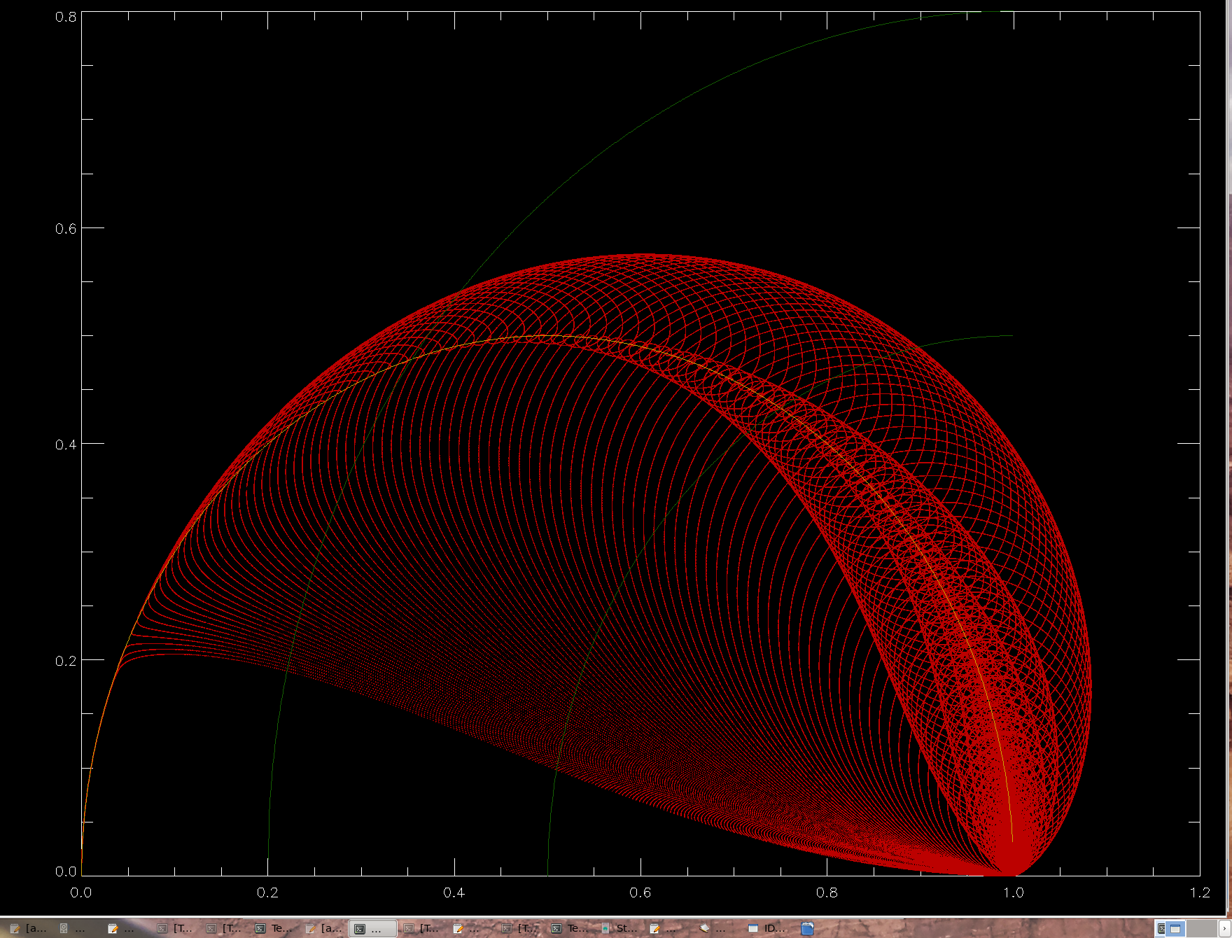
A final comment should be made about a visible change of behavior of those solutions which have a chance to approach the duck closely, i.e. for 0.9 < s < 1. The dog rushes towards the duck (lagging behind its circular motion by about 30 degrees), then slows down its approach to the duck's unit circle and turns sharply near the point M=(0.0504,0.2188) to either approach the duck very nearly along the golden path or alternatively turns RIGHT and swims toward its fixed point described above. The origin of the invisible magnet at M is totally enigmatic to your instructor, but then he hasn't read any of the historical literature on this problem. If anybody knows or can find out why the trajectories have a bifurcation near M, please let us all know. The complicated shape of trajectories certainly prevented 19. century mathematicians from finding solutions to the problem in terms of elementary functions (they do not exist). However, there is a mystery. The fixed points are quite smoothly distributed along the golden bow, with density decreasing towards its left end for obvious reasons (according to arccos function describing the angle between the duck, the dog, and the fixed point). They do not have any bifurcations or concentration points. They're oblivious to M, while the trajectories, especially the ones with dog's speed s≈0.97447, clearly are not and are ruled by something else.